Introduction

Ever since automated machine learning has entered the scene, people are asking, "Will automated machine learning replace data scientists?" I personally don't think we need to be worried about losing our jobs any time soon. Automated machine learning is great at efficiently trying a lot of different options and can save a data scientist hours of work. The caveat is that automated machine learning cannot replace all tasks. Automated machine learning does not understand context as well as a human being. This means that it may not know to create specific features that are the norm for certain tasks. Also, automated machine learning may not know when it has created things that are irrelevant or unhelpful.

To strengthen my points, I created a competition between myself and two SAS Viya tools for automated machine learning. To show that we are really better together, I combined my work with automated machine learning and compared all approaches. Before we dive into the results, let's discuss the task.

The Task

My predefined task is to predict if there are monetary costs associated with flooding events within the United States. In comparing various approaches, I will weigh ease-of-use, personal time spent, compute time, and several metrics such as Area under curve (C statistic), Gini, and Accuracy.

The data I am using comes from the NOAA Storm Events Database. I downloaded 30 years of data and appended the data together into one data set. Next, I binned similar event types together to create larger groupings of storm events. This took 68 event types down into 15 event types.

Additionally, I created a variable measuring total costs by adding all of the costs together and adding a flag for when costs are greater than 0. This binary flag will be the target variable. I then subset the data to focus only on flood events, which included flash floods, floods, and lake-shore floods. Moving forward, let's assume that all of this preparation work does not prove my usefulness yet.

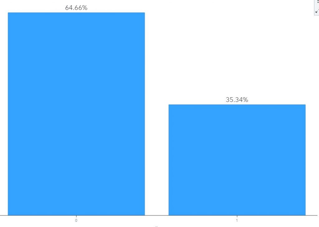
When we examine the distribution of our target below, we see that there are nearly twice as many storm events that do not have an associated cost than there are with an associated cost. Only 35% of floods accrued any cost. Following, if we predict 0 for every flood event, we will be right ~65% of the time. Thus, at a bare minimum, our models should have an accuracy greater than 0.65.

The Results

I will order my models from most-effort to least-effort.

My Best Model

To make this fair, I went through my analytical process without any automation. This means I did not use my well-loved hyperparameter autotuning or automated feature generation. I started by partitioning my data and visually exploring my data.

I created several new columns. First, I calculated how far the storm traveled using the starting coordinates and the ending coordinates. Second, I calculated how long the storm was active using the starting date-time and the ending date-time. Finally, I checked if the storm crossed zip codes, county lines, and state lines. To be perfectly honest, this feature creation took a lot of time. Translating coordinates to zip codes, counties, and states without using a paid service is not a simple task, but these variables are important to the insurance industry, so I pressed through. This effort for three new columns means that the time and effort are inflated for any method that uses these features.

To clean my data, I grouped rare values, imputed missing data and added a missing indicator, and dropped columns with high cardinality, high missingness, high consistency, or were simply not useful. Next I tried several models including a LASSO Regression, a Stepwise Regression, a Decision Tree, a Random Forest, and a Gradient Boosting model. Additionally, I adjusted various hyperparameters such as learning rate, regularization, selection, and tree-structure.

My winning model was a tuned Gradient Boosting model with stronger selection, higher learning rate, and deeper structure. Results of the process and performance are summarized in this table:

SAS Model Studio and Me

For this combined approach, I applied my knowledge of context with automated machine learning's ability to try a lot of different things. I started by taking the five features I created earlier (distance traveled, storm duration, changed zip codes, changed counties, and changed states) into Model Studio on Viya. Using Model Studio on SAS Viya, you can quickly chain together data mining preprocessing nodes, supervised learning nodes, and postprocessing nodes into a comprehensive analytics pipeline. In Model Studio, I created a pipeline using my favorite nodes and hyperparameter autotuning. Additionally, I used a provided advanced modeling template with autotuning and I asked Model Studio to create an automated machine learning pipeline. This approach took less than 10 minutes of my time to set up (after my features were already generated) and ran in the background for about 20 minutes while I completed other work.

My best performing model was an autotuned gradient boosting from the template, but all five of the variables I created were selected to be included in the model. Results of the process and performance are summarized in this table (including time for feature engineering):

Data Science Pilot and Me

Next, I combined my features with the automation of Data Science Pilot. Here, I specified to create all of the available transformations and selected the decision tree, random forest, and gradient boosting models using 5-fold validation. Writing out the SAS code took a few minutes, but running this block of code took hours. Computationally, this method took the longest, but achieved the highest model performance. Results of the process and performance are summarized in this table (including time for feature engineering):

Data Science Pilot

Following, I took the same Data Science Pilot code block and pointed it at the data set without my new features or cleaning efforts. Again, it only took a few minutes to write the code, but this method ran for hours. This approach also achieved high performance, but without my precious five features, it fell short of my previous method. Results of the process and performance are summarized in this table:

Model Studio Automated Pipeline Generation

Within SAS Model Studio on Viya, there is an option to automatically generate a pipeline within a set time limit. I removed the time limit and clicked run. This process took less than 1 minute of my time and ran in the background as I completed other tasks. Unlike Data Science Pilot, I do not have control over the various policies and parameters as the pipeline is built, which has lead to slightly different results. Results of the process and performance are summarized in this table:

Conclusion

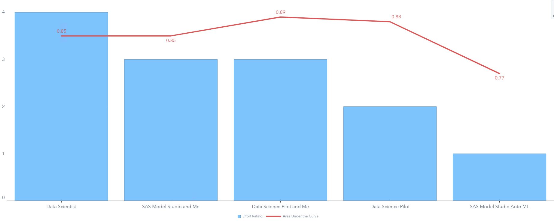
The chart above compares the Area Under the Curve (AUC) for the best performing model produced by each method with my scale of effort, with 5 being hard and 1 being easy. Our easiest method had the worst model performance, but the accuracy of this model (0.73) exceeds the minimum accuracy we defined earlier (0.65). Data Science Pilot is a powerful automation tool, and with only a few specifications, it achieved the second-best performance. But, even better performance is achieved by adding in the features I created. In conclusion, automated machine learning is a powerful tool, but it should be viewed as a complement to the data scientist rather than a competitor.

Learn More

• Maximize model performance without maximizing effort
• SAS and R Integration for Machine Learning
• SASPy for Modeling