Fitting a Neural Network Model - Learn how to fit a neural network model and use your model to score new data
In Part 6, Part 7, Part 9, and Part 10 of this series, we fit a logistic regression, decision tree, random forest and gradient boosting model to the Home Equity data we saved in Part 4. In this post we will fit a neural network model to the same data to predict who is likely to go delinquent on their home equity loan and we will score data with this model.
What is a Neural Network?
A neural network is a type of predictive modeling inspired by the way human brains process information. It consists of layers of interconnected nodes, often called neurons, that work together to analyze data and identify patterns. These networks are particularly effective at handling complex problems, such as recognizing images, predicting trends, or detecting anomalies in data.
In a neural network, data flows through multiple layers: an input layer, one or more hidden layers, and an output layer. Each layer processes the data and passes it along to the next, allowing the model to learn from the relationships within the data. Neural networks are powerful because they can adapt to the intricacies of data and make accurate predictions, even in scenarios with non-linear relationships or high-dimensional data.
What is the Neural Network Action Set?
The Neural Network Action Set in SAS Viya offers actions for building neural network models. It includes actions for fitting an artificial neural network, scoring a table with the neural network model and an action for generating DATA step scoring code. These tools enable users to create predictive models and score new data with those models.
Load the Modeling Data into Memory
Let’s start by loading our data we saved in Part 4 into CAS memory. I will load the sashdat file for my example. The csv and parquet file can be loaded using similar syntax.
conn.loadTable(path="homeequity_final.sashdat", caslib="casuser", casout={'name':'HomeEquity', 'caslib':'casuser', 'replace':True}) |
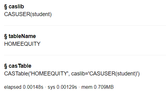
The home equity data is now loaded and ready for modeling.
Fit a Neural Network Model
Before fitting a neural network model in SAS Viya, we need to load the neuralNet action set.
conn.loadactionset(actionset="neuralNet") |
The neuralNet action set contains three actions. Let’s display the actions to see what is available for us to use.
conn.help(actionSet='neuralNet') |
The neuralNet action set includes actions for fitting a neural network and two actions for scoring using our fitted model.
Now let’s fit a neural network model with the annTrain action on the HomeEquity training data set (i.e., where _PartInd_=1). Save the model to a file named nn_model and to an astore format named nn_astore (more about this later in the post). Also specify the nominal columns in a list, assign seed the value of 1234, and specify what to use for validation data (i.e., _PartInd_ = 0). Using the validTable option allows for the validation data to be used for early stopping of the iteration process.
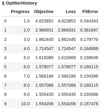
conn.neuralNet.annTrain( table = dict(name = 'HomeEquity', where = '_PartInd_ = 1'), validTable=dict(name = 'HomeEquity', where = '_PartInd_ = 0'), target = "BAD", inputs = ['LOAN','IMP_REASON','IMP_JOB','REGION','IMP_CLAGE', 'IMP_CLNO','IMP_DEBTINC','IMP_DELINQ','IMP_DEROG', 'IMP_MORTDUE','IMP_NINQ','IMP_VALUE','IMP_YOJ'], nominals = ['BAD','IMP_REASON','IMP_JOB','REGION'], seed=1234, encodeName=True, casOut = dict(name = 'nn_model', replace = True), saveState= dict(name = 'nn_astore', replace = True) ) |
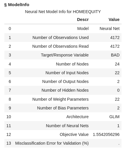
Looking at the output we can see that 1 neural network was fit with 22 input nodes and 2 output nodes, along with all the additional model info.
Let’s look at the output tables currently in memory on the CAS Server
conn.table.tableInfo() |
Score Validation Data
Like with gradient boosting we can score using the aStore file or the SAS CAS Model Table. Let’s first score the data using the aStore file.
Using the head method we can see that the data in the aStore is a binary representation.
conn.CASTable('nn_astore').head() |
Before scoring the validation data using the aStore file in SAS Viya we need to load the aStore action set.
conn.loadActionSet('aStore') |
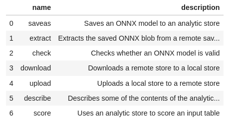
The actions in the aStore action set are listed below:
conn.builtins.help(actionSet='aStore') |
Using the score action in the aStore action set, score the validation data from the home equity data file. Use _PartInd = 0 to identify the validation rows from the data file. Create a new data set with the scored values named nn_astore_scored.
conn.aStore.score( table = dict(name = 'HomeEquity', where = '_PartInd_ = 0'), rstore = "nn_astore", out = dict(name="nn_astore_scored", replace=True), copyVars = 'BAD' ) |
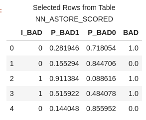
The new data has 1788 rows and 4 columns.
Use the head method to view the first five rows of nn_astore_scored file.
conn.CASTable('nn_astore_scored').head() |
In this data file, you'll find four columns, each serving a distinct purpose:
- P_BAD1: The predicted probability of an individual becoming delinquent on a home equity loan.
- P_BAD0: The complement of P_BAD1 (1 - P_BAD1), representing the predicted probability of an individual not becoming delinquent on a home equity loan.
- I_BAD: Here, you'll find the predicted classification value derived from the model.
- BAD: This column represents our target variable, acting as the label or dependent variable (Y).
For the second method lets score the validation data using the in memory scoring table nn_model. First use the head method to look at the first five rows of data. Here you can see we have rows that represent each column used in fitting the forest model.
conn.CASTable('nn_model').head() |
Now use nn_model table and the annScore action in the neuralNet action set to score the validation data (_PartInd_ = 0). Create a scored data table called nn_scored.
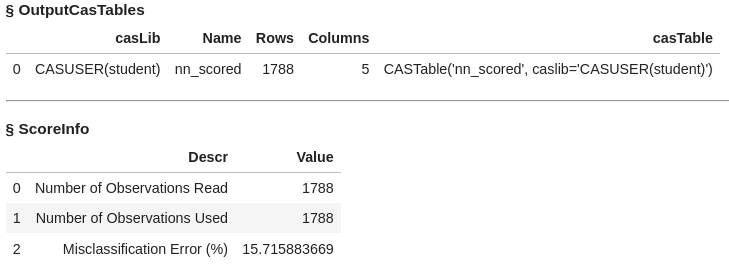
conn.neuralNet.annScore( table = dict(name = 'HomeEquity', where = '_PartInd_ = 0'), modelTable = "nn_model", casout = dict(name="nn_scored",replace=True), copyVars = ('BAD','_partind_'), encodename = True, assessonerow = True ) |
The data table nn_scored has 1788 rows and 5 columns. Output also includes the misclassification error at 15.71%
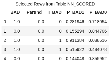
Use the head method to list the first five rows of nn_scored.
conn.CASTable('nn_scored').head() |
In this data file, you'll find five columns, each serving a distinct purpose:
- BAD: This column represents our target variable, acting as the label or dependent variable (Y).
- _PartInd_: Is the partition indicator representing the data is in the validation data with the value of 0.
- I_BAD: Here, you'll find the predicted classification value derived from the model.
- P_BAD1: The predicted probability of an individual becoming delinquent on a home equity loan.
- P_BAD0: The complement of P_BAD1 (1 - P_BAD1), representing the predicted probability of an individual not becoming delinquent on a home equity loan.
Access Model
We’ll evaluate the fit of the neural network model using the same metrics as with logistic regression, decision tree, random forest, and gradient boosting models: confusion matrix, misclassification rates, and ROC plot. These metrics will help us gauge the model’s performance and later compare it to other models.
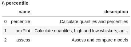
To compute these metrics, we’ll use the percentile action set along with the assess action. Start by loading the percentile action set and displaying the available actions.
conn.loadActionSet('percentile') conn.builtins.help(actionSet='percentile') |
We can use either of our scored data sets for doing assessment, as both have the same information and will give us the same output, so let’s use the nn_scored data created with the nn_model file above.
The access action creates two data sets named nn_assess and nn_assess_ROC. We can use these data sets to create the graphs and metrics for the neural network model.
conn.percentile.assess( table = "nn_scored", inputs = 'P_BAD1', casout = dict(name="nn_assess",replace=True), response = 'BAD', event = "1" ) |
Using the fetch action list the first five rows of the nn_assess dataset for inspection. You can see the values at each of the depths of data from 5% incremented by 5.
conn.table.fetch(table='nn_assess', to=5) |
Using the fetch action again on the nn_assess_ROC data, take a look at the first five rows. Here if we select cutoff of .03 the predicted true positives for our validation data would be 355 and true negatives 61. Typically, the default cutoff value is .5 or 50%.
conn.table.fetch(table='nn_assess_ROC', to=5) |
Let’s bring the output data tables to the client as data frames to calculate the confusion matrix, misclassification rate, and ROC plot for the neural network model.
nn_assess = conn.CASTable(name = "nn_assess").to_frame() nn_assess_ROC = conn.CASTable(name = "nn_assess_ROC").to_frame() |
Confusion Matrix
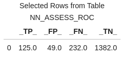
The confusion matrix can be easily calculated using the columns generated in the neural network assessment output file.
This matrix compares the predicted values to the actual values, offering a detailed breakdown of true positives, true negatives, false positives, and false negatives. These metrics provide critical insights into the model’s ability to accurately predict the target outcome.
For this analysis, a cutoff value of 0.5 will be used. If the predicted probability is 0.5 or higher, the neural network model predicts delinquency on a home equity loan. If the predicted probability is below 0.5, it predicts no delinquency. This threshold helps to evaluate the model's predictive performance systematically.
cutoff_index = round(nn_assess_ROC['_Cutoff_'],2)==0.5 conf_mat = nn_assess_ROC[cutoff_index].reset_index(drop=True) conf_mat[['_TP_','_FP_','_FN_','_TN_']] |
At the .05 cutoff value the true positives are 125 and the true negatives are 1382.
Misclassification Rate
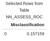
We can easily calculate the misclassification rate using the columns generated for the confusion matrix, which shows how frequently the model makes incorrect predictions.
conf_mat['Misclassification'] = 1-conf_mat['_ACC_'] miss = conf_mat[round(conf_mat['_Cutoff_'],2)==0.5][['Misclassification']] miss |
The misclassification rate of 15.71% matches the result obtained when we applied the nn_model to score the validation data.
ROC Plot
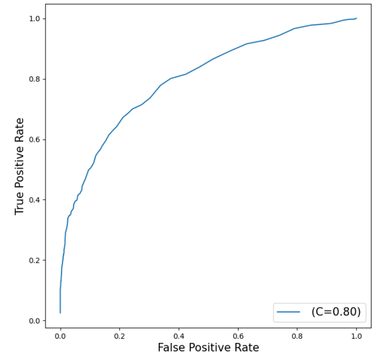
Our final assessment metric will be a ROC (Receiver Operating Characteristic) Chart, which illustrates the trade-off between sensitivity and specificity. This chart provides a comprehensive overview of the neural network model's performance, with a curve closer to the top left corner representing a more effective model.
To generate the ROC curve, use the matplotlib package in Python.
plt.figure(figsize=(8,8)) plt.plot() plt.plot(nn_assess_ROC['_FPR_'],nn_assess_ROC['_Sensitivity_'], label=' (C=%0.2f)'%nn_assess_ROC['_C_'].mean()) plt.xlabel('False Positive Rate', fontsize=15) plt.ylabel('True Positive Rate', fontsize=15) plt.legend(loc='lower right', fontsize=15) plt.show() |
The curve generated by the neural network model does not fit the data as well as the gradient boosting model, which achieved a more effective fit with an AUC of 0.96. While the neural network curve is still above the diagonal, it is farther from the top left corner, indicating that there is significant room for improvement.
The AUC (Area Under the Curve) value for the neural network is 0.80. This suggests the model performs better than a random classifier, which would have an AUC of 0.5. However, it falls short of the ideal scenario of an AUC of 1, which would represent a perfect model. Compared to the gradient boosting model, the neural network's performance highlights the importance of selecting the right algorithm for the dataset and problem at hand.
The Wrap-Up: Fitting a Neural Network Model
In this post, we explored how to fit a neural network model using the SAS Viya SWAT package and evaluated its performance with metrics such as the confusion matrix, misclassification rates, and ROC plots. While the neural network achieved an AUC of 0.80, indicating it performed better than a random classifier, it did not match the gradient boosting model’s higher AUC of 0.96. This underscores the importance of comparing multiple algorithms to find the best fit for your data.
In the next blog post, we’ll focus on fitting a support vector machine (SVM) model to the same data to predict delinquency on home equity loans. Stay tuned to see how the SVM model compares to the other models we've explored so far.
