Learn how to fit a decision tree and use your decision tree model to score new data.
In Part 6 of this series we took our Home Equity data saved in Part 4 and fit a logistic regression to it. In this post we will use the same data and fit a classification decision tree to predict who is most likely to go delinquent on their home equity loan.
For fitting decisions trees we will use the decisiontree action set and the dtreeTrain action and use the dtreeScore action to score our validation data.
What is a Decision Tree?
A decision tree is a representation of possible outcomes based on a series of decisions or variables. It is commonly used in data analysis and predictive modeling to help understand and interpret complex relationships within the data.
A decision tree is created through a process called recursive partitioning, which uses an algorithm to split the data into smaller and more homogenous groups based on specific variables. This allows for the identification of key patterns and relationships within the data, forming branches and nodes in the decision tree.
What is the Decision Tree Action Set?
With SAS Viya, you can easily build, train, and evaluate decision trees to make accurate predictions and informed decisions based on your data using the Decision Tree Action Set.
What is a Classification Tree vs a Regression Tree?
There are two main types of decision trees: classification and regression. Classification trees are used for predicting categorical or discrete outcomes, while regression trees are used for predicting continuous outcomes.
For our example we will be fitting a classification tree since BAD is a classification variable with 2 levels. 0 if the person is not delinquent on their home equity loan and 1 if they are delinquent.
Load the Modeling Data into Memory
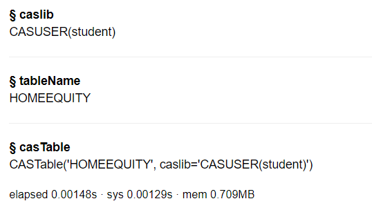
Let’s start by loading our data, the sashdat, csv, and parquet files we saved in part 4 into CAS memory. I will load the sashdat file using the code below. The csv and parquet file can be loaded using similar syntax.
conn.loadTable(path="homeequity_final.sashdat", caslib="casuser", casout={'name':'HomeEquity', 'caslib':'casuser', 'replace':True}) |
The home equity data is now loaded and ready for modeling.
Fit a Decision Tree
Before fitting a decision tree in SAS Viya we need to load the decisionTree action set.
conn.loadActionSet('decisionTree') |
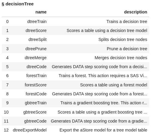
The decisionTree action set contains several actions, let’s display the actions to see what is available for us to use.
conn.help(actionSet='decisionTree') |
This action set not only contains actions for fitting and scoring decision trees but also for fitting and scoring random forest models and gradient boosting models. Examples for fitting these two will be included in future posts.
Fit a decision tree using the the dtreeTrain action using the HomeEquity training data set (ie where _PartInd_=1). Save the model to a file named dt_model. We will use a split criterion of information gain and prune equal to true to use C4.5 pruning method. Also specify the variable importance information to be generated.
Assign the results to Tree_Output.
Tree_Output = conn.decisionTree.dtreeTrain( table = dict(name = HomeEquity, where = '_PartInd_ = 1'), target = 'BAD', inputs = ['LOAN', 'IMP_REASON', 'IMP_JOB' ,'REGION', 'IMP_CLAGE', 'IMP_CLNO', 'IMP_DEBTINC', ‘IMP_DELINQ', 'IMP_DEROG', 'IMP_MORTDUE', 'IMP_NINQ', 'IMP_VALUE', 'IMP_YOJ'], nominals = ['BAD','IMP_REASON','IMP_JOB','REGION'], casOut = dict(name='dt_model', replace = True), crit="GAIN", prune=True, varImp=True ) |
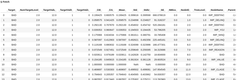
Let’s take a look at what the data looks like in the model file dt_model generated from our decision tree.
conn.CASTable("dt_model").fetch() |
What are the keys created as part of the output in Tree_Output?
list(Tree_Output.keys()) |
Three keys are created.
![]()
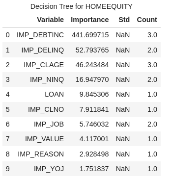
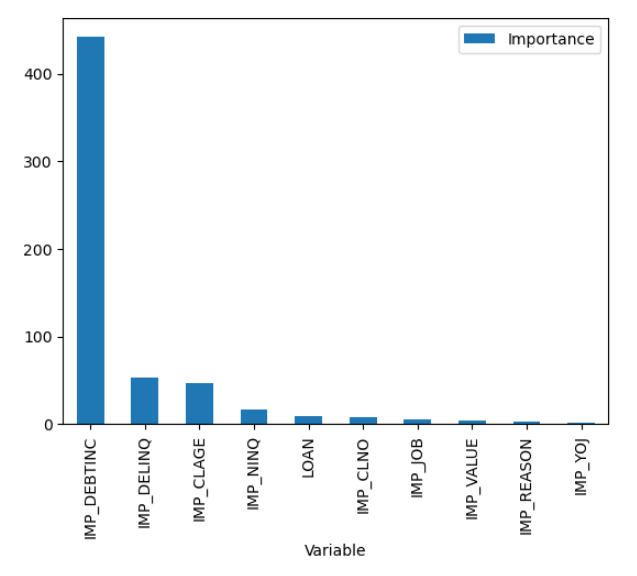
Let’s look at the important variable information generated for our decision tree model. 9 of our 14 variables turned out to be important in our model and the list below shows them in the order of importance.
Tree_Output['DTreeVarImpInfo'] |
Now plot these values by creating a data frame with this table and using the Python package matplotlib.
from matplotlib import pyplot as plt df = Tree_Output['DTreeVarImpInfo'] df.plot(kind = 'bar', x = 'Variable', y = 'Importance') |
Score Validation Data
Now let’s take the model created (file named dt_model) and score using the dtreeScore action to apply it to the validation data (_PartInd_=0). Create a new dataset called dt_scored to store the scored data.
dt_score_obj = conn.decisionTree.dtreeScore( table = dict(name = HomeEquity, where = '_PartInd_ = 0'), model = "dt_model", casout = dict(name="dt_scored",replace=True), copyVars = 'BAD', encodename = True, assessonerow = True ) |
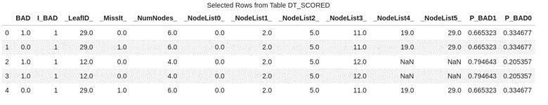
Look at the first five rows of the scored data to see the predicted probability for each row.
conn.CASTable('dt_scored').head() |
Access Model
We will assess the performance of a decision tree model using the same metrics we used for the logistic regression in Part 6 of this series: confusion matrix, misclassification rates, and a ROC (Receiver Operating Characteristic) plot. These measures help us determine how well our decision tree model fits the data.
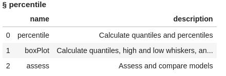
To calculate these metrics, we will use the percentile action set and the assess action. Load the percentile action set and display the actions.
conn.loadActionSet('percentile') conn.builtins.help(actionSet='percentile') |
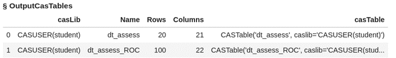
Assess the decision tree model using the scored data (dt_scored). Two data sets are created name dt_assess and dt_assess_ROC.
conn.percentile.assess( table = "dt_scored", inputs = 'P_BAD1', casout = dict(name="dt_assess",replace=True), response = 'BAD', event = "1" ) |
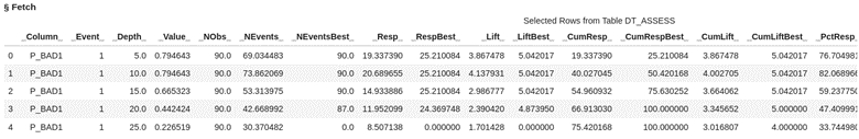
Look at the first five rows of the data from the assess action output dataset dt_assess. Here you see the values at each of the depths of data from 5% incremented by 5.
display(conn.table.fetch(table='dt_assess', to=5)) |
Look at the first five rows of data from the assess action output data set dt_assess_ROC. This data is organized by cutoff value starting .00 and going to 1 incremented by the value of .01.
conn.table.fetch(table='dt_assess_ROC', to=5) |
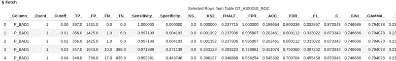
In decision trees, like in logistic regression, we use a cutoff value to make decisions, kind of like drawing a line in the sand. In this case if we use a cutoff value of .03 using the table above it means we are using the prediction probability of .03 to predict if someone is going to be delinquent on their loan. If we choose .03 then for our validation data the predicted true positives will be 347 and true negatives 388. The default cutoff value is .5 or 50%.
Bring these results to our client by creating local data frames so we can calculate a confusion matrix, misclassification rate, and ROC plot for our decision tree model.
dt_assess = conn.CASTable(name = "dt_assess").to_frame() dt_assess_ROC = conn.CASTable(name = "dt_assess_ROC").to_frame() |
Confusion Matrix
Create a confusion matrix, which compares predicted values to actual values. It breaks down these predictions into four categories: true positives, true negatives, false positives, and false negatives. Here are the category definitions:
- A true positive happens when the actual value is 1 and our model predicts a 1.
- A false positive is when the actual value is 0 and our model predicts a 1.
- A true negative is when the actual value is 0 and our model predicts a 0.
- A false negative is when the actual value is a 1 and our model predicts a 0.
These measures help us evaluate the performance of the model and assess its accuracy in predicting the outcome of interest.
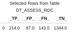
Use a cutoff value of 0.5, which means if the predicted probability is greater than or equal to 0.5 then our model predicts someone will be delinquent on their home equity loan. If the predicted value is less than 0.5 then our model predicts someone will not be delinquent on their home equity loan.
#create confusion matrix cutoff_index = round(dt_assess_ROC['_Cutoff_'],2)==0.5 conf_mat = dt_assess_ROC[cutoff_index].reset_index(drop=True) conf_mat[['_TP_','_FP_','_FN_','_TN_']] |
Misclassification Rate
We can also calculate a misclassification rate, which indicates how often the model makes incorrect predictions.
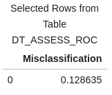
# calculate misclassification rate conf_mat['Misclassification'] = 1-conf_mat['_ACC_'] miss = conf_mat[round(conf_mat['_Cutoff_'],2)==0.5][['Misclassification']] miss |
Our misclassification rate for our decision tree model is .128635 or 13%. This means that our model is wrong 13% of the time, but correct 87%.
ROC Plot
Additionally, a ROC (Receiver Operating Characteristic) plot visually displays the trade-off between sensitivity and specificity, helping us evaluate the overall performance of the model. The closer the curve is to the top left corner, the higher the overall performance of the model.
Use the Python graphic package matplotlib to plot our ROC Curve.
# plot ROC Curve from matplotlib import pyplot as plt plt.figure(figsize=(8,8)) plt.plot() plt.plot(dt_assess_ROC['_FPR_'],dt_assess_ROC['_Sensitivity_'], label=' (C=%0.2f)'%dt_assess_ROC['_C_'].mean()) plt.xlabel('False Positive Rate', fontsize=15) plt.ylabel('True Positive Rate', fontsize=15) plt.legend(loc='lower right', fontsize=15) plt.show() |
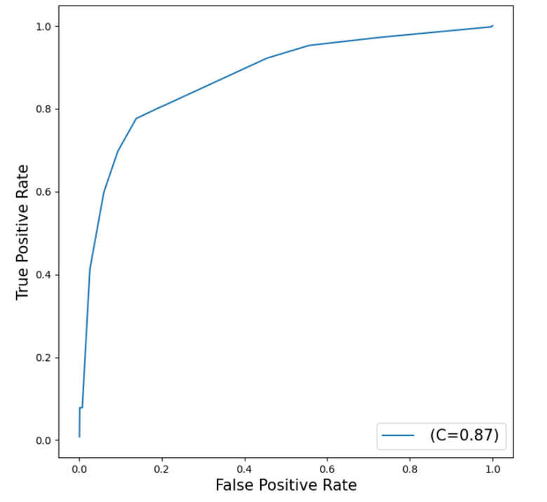
Our curve is somewhat close to the top left corner which indicates a good fit, but also shows room for improvement. The C=0.87 represents the Area Under the Curve (AUC) statistic which means our model is doing better than the 0.5 of a random classifier but not as good as the perfect model at 1.
The Wrap-Up: Fitting a Decision Tree
The Decision Tree action set in SAS Viya with Python using SWAT makes it simple to create and analyze decision trees for your data. Using the dtreeTrain to train our decision tree and dtreeScore to score our validation or hold out sample we can evaluate how well our decision tree model fits our data and predicts new data.
In the next post, we will learn how to compare the logistic regression model to this decision tree for assessing which of these two models is the best model between the two.
Related Resources
SAS Help Center: Load a SASHDAT File from a Caslib
SAS Help Center: loadTable Action
Getting Started with Python Integration to SAS® Viya® - Part 5 - Loading Server-Side Files into Memory
SAS Help Center: Decision Tree Details
SAS Help Center: dtreeTrain Action
SAS Help Center: dtreeScore Action
SAS Help Center: Percentile Action Set
SAS Help Center: assess Action
Tree-related Models: Supervised Learning in SAS Visual Data Mining and Machine Learning
Decision Tree in Layman’s Terms - SAS Support Communities