Learn how to split your data into a training and validation data set to be used for modeling.
In part 3 of this series, we replaced the missing values with imputed values. Our final step in preparing the data for modeling is to split the data into a training and validation data set. This is important so that we have a set of data to train the model and a holdout or separate set of data to validate the model and make sure it performs well with new data.
For this step we will use the sampling action set and will show examples using both the srs (simple random sampling) and stratified actions.
Why is it Important to Create Training and Validation Data Sets
When it comes to data modeling, having both training and validation datasets is essential for ensuring the accuracy and reliability of our models. The training dataset is used for training the model on a portion of the data, while the validation dataset is used to assess the performance of the trained model on a holdout sample of the data. This process of splitting data into two separate sets helps prevent overfitting and helps us understand how well the model generalizes to new data.
Having a validation dataset allows us to evaluate our models objectively and adjust if necessary. It also helps us avoid the mistake of assuming that a model that performs well on the training data will also perform well on a holdout sample of the data. Without proper validation, we may end up with a model that is biased towards the training data and performs poorly on new data.
Furthermore, having a separate validation dataset allows us to fine-tune our model and select the best performing one before deploying it in a real-world scenario. This can save time, resources, and potential consequences of using an inadequate model. In summary, incorporating both training and validation datasets into our modeling process is crucial for enhancing accuracy, reliability, and generalization of our models.
What is the Sampling Action Set?
The sampling action set allows us to sample data in SAS Viya. It consists of four actions: srs, stratified, oversampling, and k-fold. Let's look at examples for srs and stratified in this post.
The sampling action set in our example will create an output table including a variable identifying the partition or sample the row or observations belongs to. The partition variable name is _Partind_.
The training data is identified when _Partind_ = 1 and the validation data is identified when _Partind_=0.
What is SRS?
Simple random sampling (SRS) is like picking names out of a hat. Just like how you give everyone an equal chance to be picked when playing a game, SRS gives every item in a group an equal chance of being selected for the sample. This helps us get a fair representation of the whole group without leaving anyone out.
What is Stratified?
Stratified sampling is like sorting candy into different groups like chocolate vs non-chocolate before picking a few from each group to eat. Just like how we might want to try all the different types of candy, stratified sampling allows us to get a fair representation of each group in a population by selecting some from each group for our sample. This helps us get a more accurate understanding of the whole population.
Let’s Assign Rows to be in Training and Validation Data
For the Home Equity data, we want to create training data that includes 70% of the data and the validation will include the remaining 30%. So, for our data we want to have _Partind_ randomly assigned the value of 1 to 70% and the value of 2 to 30% of the rows.
Using the sampling action set with the srs action, our code looks like this where the samppct represents the 70 percent of the data we want to be used for training. We also want _Partind_ indicator variable created to identify which row is in the training vs validation data. Finally, the seed is a number we select (and can be any integer value) so that we can replicate the results.
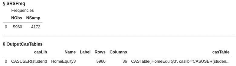
conn.loadActionSet('sampling') conn.sampling.srs( table = 'HomeEquity2', samppct = 70, seed = 919, partind = True, output = dict(casOut = dict(name = 'HomeEquity3', replace = True), copyVars = 'ALL') ) |
For our data the srs action has taken the original 5,960 rows and assigned 4,172 to be in the training data, so for these 4,172 the _Partind_=1.
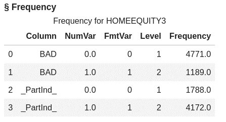
Let’s look at the count in each partition for training and validation using the freq action in the simple action set.
conn.simple.freq( table = 'HomeEquity3', inputs = ["BAD","_Partind_"] ) |
Here we can see for the _Partind_ indicator variable that we have the correct assignment of 4,172 rows.
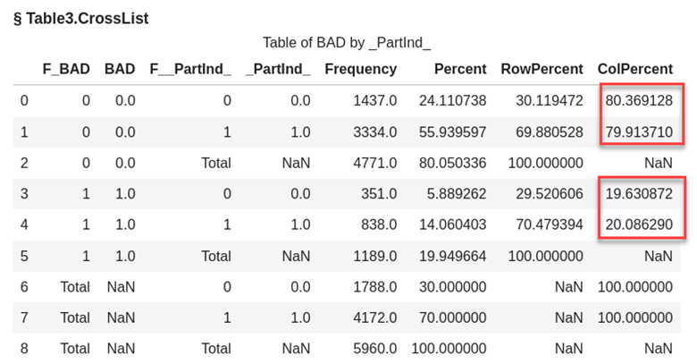
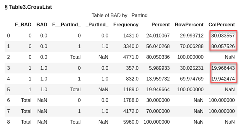
Does this sample represent the number of people that went delinquent on their home equity loan fairly in the training and validation data? Let’s use the freqTab action to look at a crosstab of the number of people who when delinquent (BAD) and _Partind_ to compare the percentages in the groups.
conn.freqTab(table="HomeEquity3", tabulate=['BAD','_Partind_',{'vars':{'BAD','_Partind_'}}] ) |
From the highlighted column percentages in the output table we see that the percentages are close but not exact. To have BAD equally represented in the training and validation data we would need to use stratified sampling instead of SRS.
Using the stratified action in the sampling action set we will also need to use the groupby option to specify BAD as our stratification variable.
conn.sampling.stratified( table = {'name':'HomeEquity2', 'groupby' : 'bad'}, samppct = 70, seed = 919, partind = True, output = dict(casOut = dict(name = 'HomeEquity4', replace = True), copyVars = 'ALL') ) |
In our output for the stratified sample, we still have a 70% sample or 4,172 rows assigned to our training data but now the proportion of BAD is better represented.
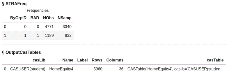
As you can see in the output below highlighted in red from the freqTab action the percentages are now almost identical.
We are happy with our data and are now ready to create some models. Let’s save the data so we have all our updates available for our modelers.
Save the final modeling dataset
We will not use all the columns in the data so to be efficient for storage and modeling, we will specify the columns to save. For example, we will be using the imputed columns and will not need the original for our models.
For the next step, determine the columns for inclusion in the modeling dataset. Use the alterTable action in the table action set to keep the columns for modeling and to create the order of the columns in the data.
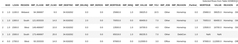
Next, verify the desired outcome by printing the first 5 rows.
## Reference the new CAS table and reorganize columns finalTbl = conn.CASTable('HomeEquity4', caslib = 'casuser') ## Specify the order of the columns newColumnOrder = ['BAD', 'LOAN', 'REGION', 'IMP_CLAGE', 'IMP_CLNO', 'IMP_DEBTINC', 'IMP_DELINQ', 'IMP_DEROG', 'IMP_MORTDUE', 'IMP_NINQ', 'IMP_VALUE', 'IMP_YOJ', 'IMP_JOB', 'IMP_REASON', '_PartInd_'] finalTbl.alterTable(keep = {'BAD', 'LOAN', 'REGION', 'IMP_CLAGE', 'IMP_CLNO', 'IMP_DEBTINC', 'IMP_DELINQ', 'IMP_DEROG', 'IMP_MORTDUE', 'IMP_NINQ', 'IMP_VALUE', 'IMP_YOJ', 'IMP_JOB', 'IMP_REASON', '_PartInd_'}) finalTbl.alterTable(columnOrder = newColumnOrder) ## Preview the CAS table finalTbl.head() |
First 5 rows of the data looks great!
Our data table is now ready for us to create models. Let’s save it to a file using the table.save CAS action so we can load it into memory later for our modeling activities.
You can decide if you want to save the data as a .sashdat file
finalTbl.save(name = 'homeequity_final.sashdat', caslib = 'casuser') |
or a csv file
finalTbl.save(name = 'homeequity_final.csv', caslib = 'casuser') |
or parquet file type.
finalTbl.save(name = 'homeequity_final.parquet', caslib = 'casuser') |
For more information about saving files check out Getting Started with Python Integration to SAS® Viya® - Part 17 - Saving CAS tables blog post.
The Wrap-Up: Creating Training and Validation Data Sets
We have learned the importance of preparing our data before beginning the modeling process. Through the first four parts of this series by exploring and understanding our data, handling missing values, and creating training and validation datasets, we have set ourselves up for success in our modeling endeavors. By following these steps, we can confidently move on to the next part of this series and begin the exciting task of building models to gain insights and make predictions.
In the next post, we will learn how to fit a Linear Model using the data we prepared and saved.