Learn how to fit a logistic regression and use your model to score new data.

In part 4 of this series, we created and saved our modeling data set with all our updates from imputing missing values and assigning rows to training and validation data. Now we will use this data to predict if someone is likely to go delinquent on their home equity loan.

Just like in Part 5, where we fit a linear regression to this data, we will be using the regression action set, but this time with the logistic action. Then we will take our model and score the validation data using the logisticScore action.

What is Logistic Regression?

Logistic regression is a statistical technique for predicting binary outcomes (e.g., yes or no to being delinquent on a home equity loan) based on one or more independent variables. It works by estimating the probability of an event occurring and classifying it as either 0 or 1, making it useful for predicting categorical outcomes. It is commonly used in fields such as medicine, marketing, and finance to analyze and understand the relationship between predictor variables and a binary outcome.

What is the Regression Action Set?

The Regression Action Set in SAS Viya is a collection of procedures and functions designed to perform various types of regression analysis. It includes actions such as Linear Regression, Logistic Regression, General Linear Models (GLM), and more. These actions allow users to build statistical models for predicting outcomes or understanding the relationships between variables. Additionally, the action set provides various options for model selection, diagnostics, and scoring, helping users interpret and validate their results. Overall, the Regression Action Set in SAS Viya offers a comprehensive set of tools for conducting regression analysis efficiently and effectively.

To fit a logistic regression and score data we will use the logistic action and the logisticScore action from the Regression Action Set.

Load the Modeling Data into Memory

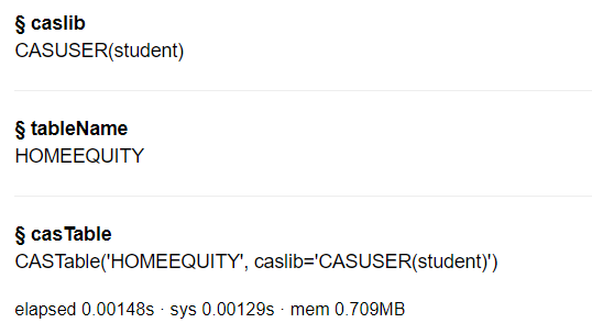
Let’s start by loading our data we saved in part 4 into CAS memory. I will load the sashdat file for my example. The csv and parquet file can be loaded using similar syntax.

conn.loadTable(path="homeequity_final.sashdat", caslib="casuser",
               casout={'name':'HomeEquity',
                               'caslib':'casuser', 'replace':True})

The home equity data is now loaded and ready for modeling.

Fit Logistic Regression

Before we can fit a logistic regression model, we need to load the regression action set.

conn.loadActionSet('regression')

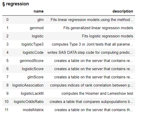
The regression action set consists of several actions, let’s display the actions in the regression action set to see what is available.

conn.help(actionSet='regression')

The actions include modeling algorithms like glm, genmod, and logistic as well as corresponding actions where we can score data using the models created.

Fit a logistic regression model using logistic action on the HomeEquity training data set (ie where _PartInd_ =1). Save the model to a file named lr_model. In the model statement we also indicate to fit the model to those who went BAD (or delinquent) on their loan (i.e., event=1)

conn.regression.logistic( 
    table = dict(name = HomeEquity, where = '_PartInd_ = 1'), 
    classVars=['IMP_REASON','IMP_JOB','REGiON'],
    model=dict(depVar=[dict(name='BAD', options=dict(event='1'))], 
                          effects=[dict(vars=['LOAN', 'IMP_REASON', 'IMP_JOB', 'REGiON',  'IMP_CLAGE',  
                                        'IMP_CLNO', 'IMP_DEBTINC', 'IMP_DELINQ', 'IMP_DEROG',  
                                        'IMP_MORTDUE', 'IMP_NINQ', 'IMP_VALUE', 'IMP_YOJ'])]
                          ),
    store = dict(name='lr_model',replace=True)
)

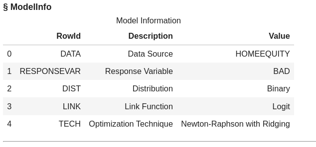
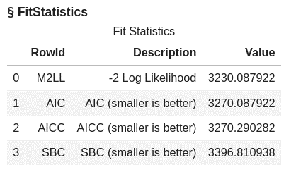
The default output includes information about the model, the number of observations used, response profile, class level information, convergence status, fit statistics, and parameter estimates.

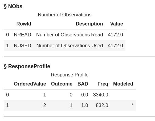
The data used was the HomeEquity data we loaded in memory and the target variable or Y is BAD, which is the 0, 1 indicator variable on whether someone went delinquent on a home equity loan. 4,172 rows from the training data were used to train the model.

The asterisk in the image below indicates that BAD=1 was the level modeled for this logistic regression.

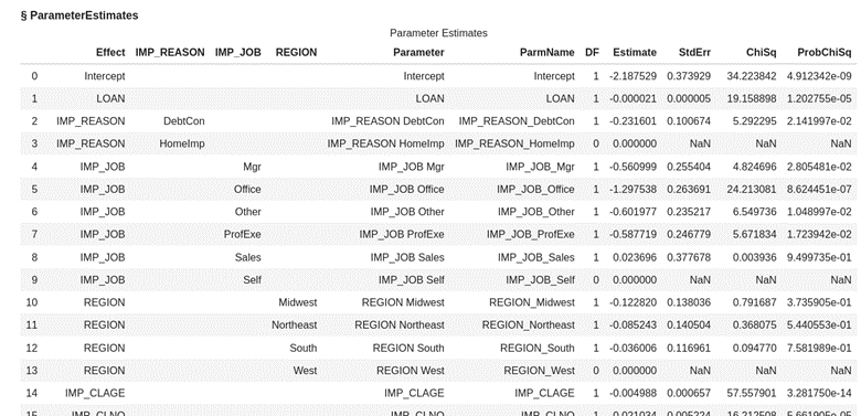
Partial list of parameters from the logistic regression model fitted (or trained) is shown below.

Score Validation Data

Now let’s take the model created (file named lr_model) and score it using the logisticScore action to apply it to the validation data (_PartInd_=0). Create a new dataset called lr_scored to store the scored data.

lr_score_obj = conn.regression.logisticScore( 
    table = dict(name = HomeEquity, where = '_PartInd_ = 0'), 
    restore = "lr_model", 
    casout = dict(name="lr_scored", replace=True), 
    copyVars = 'BAD',
    pred='P_BAD')

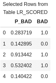
Look at first 5 rows of the scored data to see the predicted probability for each row and the actual value of BAD.

conn.CASTable('lr_scored').head()

Assess the Model

To assess the performance of a logistic regression model, we can use metrics such as a confusion matrix, misclassification rates, and a ROC (Receiver Operating Characteristic) plot. These measures can help us determine how well our logistic regression model fits the data and make any necessary adjustments to improve its accuracy.

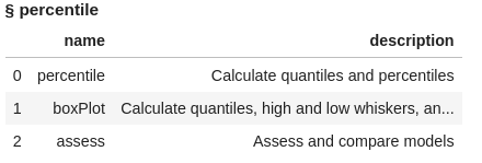
To calculate these metrics, we will use the percentile action set and the assess action. Load the percentile action set.

conn.loadActionSet('percentile')
conn.builtins.help(actionSet='percentile')

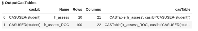
Assess the logistic regression model using the scored data (lr_scored). Two data sets are created named lr_assess and lr_assess_ROC

conn.percentile.assess(
   table = "lr_scored",
   inputs = 'P_BAD',
   casout = dict(name="lr_assess", replace=True),
   response = 'BAD',
   event = "1"
)

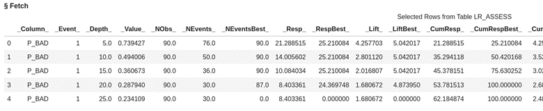
Look at the first 5 rows of data from the assess action output data set lr_assess. Here you see the values at each of the depths of data from 5% incremented by 5.

display(conn.table.fetch(table='lr_assess', to=5))

Look at the first 5 rows of data from the assess action output data set lr_assess_ROC. This data is organized by cutoff value starting .00 and going to 1 incremented by the value of .01.

conn.table.fetch(table='lr_assess_ROC', to=5)

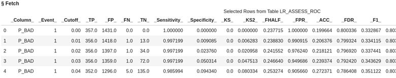
In logistic regression, we use a cutoff value to make decisions, kind of like drawing a line in the sand.
In this case if we use a cutoff value of .03 using the table below it means we are using the prediction probability of .03 to predict if someone is going to be delinquent on their loan. If we choose .03 then for our validation data the predicted true positives will be 356 and true negatives 72. The default cutoff value is .5 or 50%.

Let's now bring the results to client by creating local data frames to calculate a confusion matrix, misclassification rate, and ROC plot for our logistic regression model.

lr_assess = conn.CASTable(name = "lr_assess").to_frame()
lr_assess_ROC = conn.CASTable(name = "lr_assess_ROC").to_frame()

Create a confusion matrix, which compares predicted values to actual values. It breaks down these predictions into four categories: true positives, true negatives, false positives, and false negatives. A true positive happens when the actual value is 1 and our model predicts a 1. A false positive is when the actual value is 0 and our model predicts a 1. A true negative is when the actual value is 0 and our model predicts a 0. A false negative is when the actual value is a 1 and our model predicts a 0.

These measures help us evaluate the performance of the model and assess its accuracy in predicting the outcome of interest.

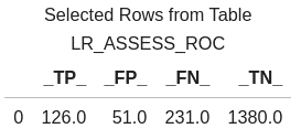
Use a cutoff value of 0.5, which means if the predicted probability is greater than or equal to 0.5 then our model predicts someone will be delinquent on their home equity loan. If the predicted value is less than 0.5 then our model predicts someone will not be delinquent on their home equity loan.

# create confusion matrix
cutoff_index = round(lr_assess_ROC['_Cutoff_'],2)==0.5
conf_mat = lr_assess_ROC[cutoff_index].reset_index(drop=True)
conf_mat[['_TP_','_FP_','_FN_','_TN_']]

We can also calculate a misclassification rate, which indicates how often the model makes incorrect predictions.

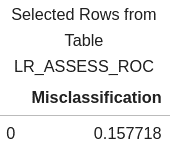
# calculate misclassification rate
conf_mat['Misclassification'] = 1-conf_mat['_ACC_']
miss = conf_mat[round(conf_mat['_Cutoff_'],2)==0.5][['Misclassification']]
miss

Our misclassification rate for our logistic regression model is .157718 or 16%. This means that our model is wrong 16% of the time, but correct 84%.

Additionally, a ROC (Receiver Operating Characteristic) plot visually displays the trade-off between sensitivity and specificity, helping us evaluate the overall performance of the model. The closer the curve is to the top left corner, the higher the overall performance of the model.

Use the Python graphic package matplotlib to plot our ROC Curve.

# plot ROC Curve
from matplotlib import pyplot as plt
 
plt.figure(figsize=(8,8))
plt.plot()
 
plt.plot(lr_assess_ROC['_FPR_'],lr_assess_ROC['_Sensitivity_'], label=' (C=%0.2f)'%lr_assess_ROC['_C_'].mean())
 
plt.xlabel('False Positive Rate', fontsize=15)
plt.ylabel('True Positive Rate', fontsize=15)
plt.legend(loc='lower right', fontsize=15)
plt.show()

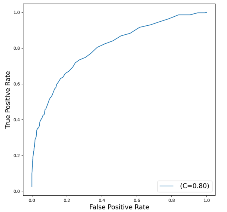
Our curve is somewhat close to the top left corner which indicates a good fit, but also shows room for improvement.

The C=0.8 represents the Area Under the Curve (AUC) statistic which means our model is doing better than the 0.5 of a random classifier but not as good as the perfect model at 1.

The Wrap-Up: Fitting a Logistic Regression

Logistic regression is a powerful tool in SAS Viya for predicting binary outcomes. By using the regression action set with the logistic action, we can build and assess various models to find the best fit for our data. We can also utilize the logisticScore action to score data with the percentile action set to assess our model using criterion like confusion matrixes, misclassification rate, and ROC curves to evaluate and compare different models. This ultimately aids us in making accurate predictions and informed decisions based on our data.

In the next post, we will learn how to fit a decision tree to our Home Equity Data.

Related Resources

SAS Help Center: Load a SASHDAT File from a Caslib
SAS Help Center: loadTable ActionGetting Started with Python Integration to SAS® Viya® - Part 5 - Loading Server-Side Files into Memory
SAS Help Center: Regression Action Set
SAS Help Center: logistic Action
SAS Help Center: logisticScore Action
SAS Help Center: Percentile Action Set
SAS Help Center: assess Action