Learn how to fit a linear regression and use your model to score new data.

In part 4 of this series, we created our modeling dataset by including a column to identify the rows to be used for training and validating our model. Here, we will create our first model using this data.

In this example, we will fit a linear model on the training data using the regression action set with the glm action. Then, we will take our model and score the validation data using the glmScore action.

What is Linear Regression?

Linear regression is a statistical method used to identify and analyze the relationship between one or more independent variables (x or features) and a dependent variable (y, target, or label). It is often used in data analysis to predict numeric values based on historical trends and patterns, making it a valuable tool for decision-making.

By using linear regression, we can better understand the impact of different factors on our desired outcome and make more informed decisions. Additionally, it allows us to quantify the strength and direction of relationships between variables, providing valuable insights into our data. So, in summary, linear regression is an essential tool for understanding and making sense of complex data sets.

What is the Regression Action Set?

The regression action set in SAS Viya is a collection of procedures and functions designed to perform various types of regression analysis. It includes actions such as linear regression, logistic regression, general linear models (GLM), and more. These actions allow users to build statistical models that predict outcomes or understand the relationships between variables.

Additionally, the action set provides various options for model selection, diagnostics, and scoring to help users interpret and validate their results. Overall, the regression action set in SAS Viya offers a comprehensive set of tools for conducting regression analysis efficiently and effectively.

What is GLM?

GLM stands for general linear models, and it is a type of regression analysis that fits linear regression models using the method of least squares.

Load the Modeling Data into Memory

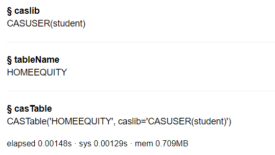
Let’s start by loading our data we saved in part 4 into CAS memory. I will load the sashdat file for my example. The csv and parquet file can be loaded using similar syntax.

conn.loadTable(path="homeequity_final.sashdat", caslib="casuser",
               casout={'name':'HomeEquity',
                               'caslib':'casuser', 'replace':True})

The home equity data is now loaded and ready for modeling.

Fit a Linear Regression Model

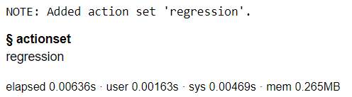
Before we can fit a linear regression model, we need to load the regression action set.

conn.loadActionSet('regression')

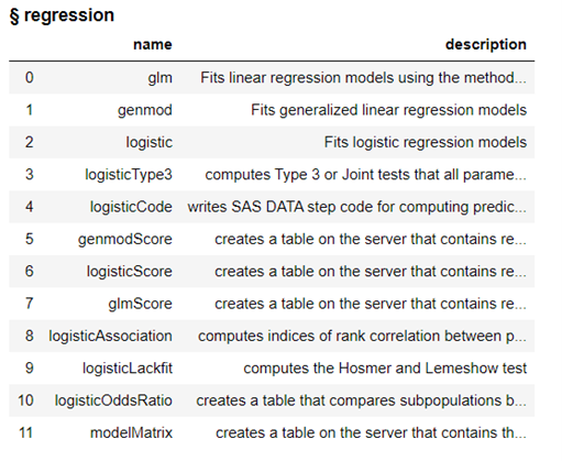
The regression action set consists of several actions, let’s display the actions in the regression action set to see what is available.

conn.help(actionSet='regression')

The actions include modeling algorithms like glm, genmod, and logistic as well as corresponding actions where we can score data using the models created.

Fit a linear regression model using the glm action on the HomeEquity training data set (i.e., where _PartInd_=1). Save the model to a file named reg_model.

conn.regression.glm(
    table= dict(name = HomeEquity, where = '_PartInd_ = 1'),
    classVars=['IMP_REASON','IMP_JOB','REGION','BAD'],
    model={'depVar':'LOAN',
                   'effects':['IMP_REASON', 'IMP_JOB', 'REGION', 'BAD', 'IMP_CLAGE', 'IMP_CLNO',  
                    'IMP_DEBTINC', 'IMP_DELINQ', 'IMP_DEROG', 'IMP_MORTDUE', 'IMP_NINQ',
                    'IMP_VALUE', 'IMP_YOJ']
                  },
    store = dict(name='reg_model', replace=True)
)

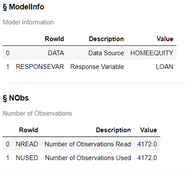
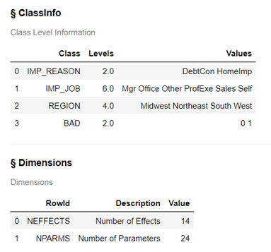
The output includes information about the model, the number of observations used, classification variables, ANOVA, fit statistics, and parameter estimates.

The HomeEquity data we loaded earlier into memory was used and the target variable or Y is LOAN, which is the amount of the home equity loan. The 4,172 rows from the training data were used to train the model.

For the classification variable IMP_REASON and BAD each have 2 levels (or values), REGION has 4, and IMP_JOB has 6. The model has 14 effects (or inputs) and 24 parameters were estimated.

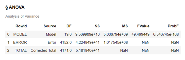
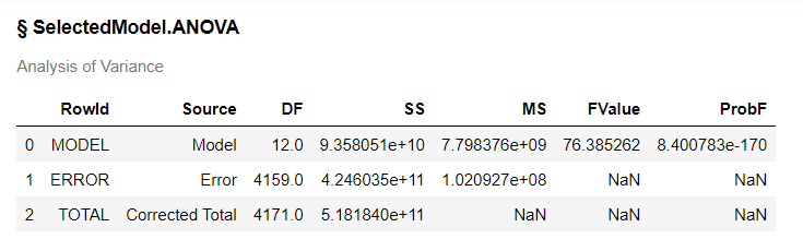
The Analysis of Variance (ANOVA) table shows overall statistics about the linear model created.

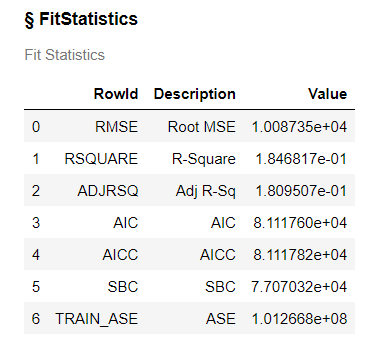
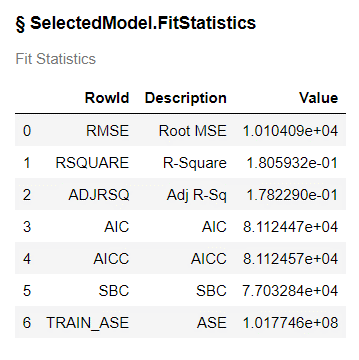
The fit statistics give us an overall understanding on how well the model fits the data and allows us to compare this model to other models to determine which is better at fitting the data.

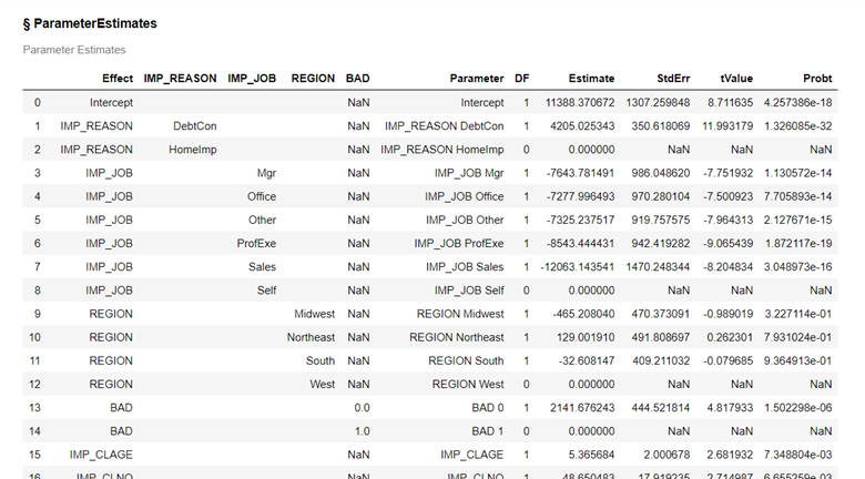
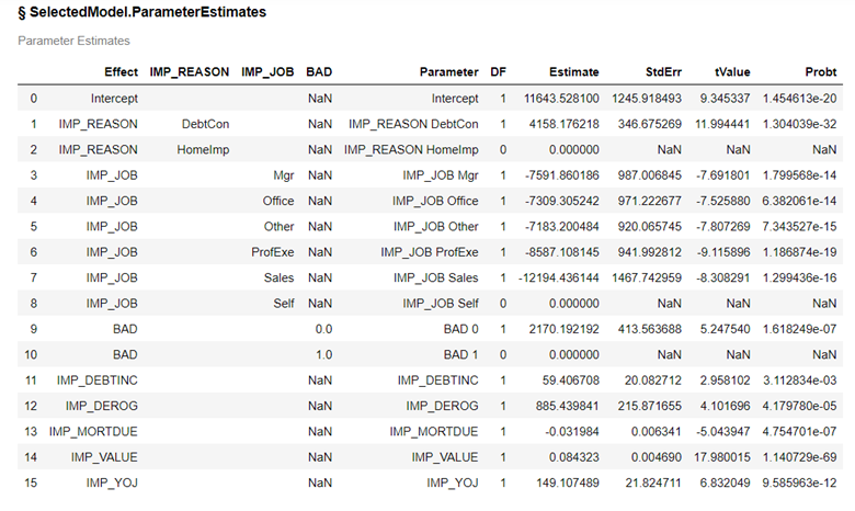
This is a partial list of parameter estimates for our model.

Score Validation Data

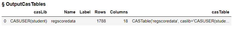
Now take the model created (file named reg_model) and score using the glmScore action to apply it to the validation data (_PartInd_=0). Create a new dataset called regscoredata to store the scored data.

conn.regression.glmScore(
    table= dict(name = HomeEquity, where = '_PartInd_ = 0'),
    restore='reg_model',
    casOut=dict(name='regscoredata', replace=True),
    fitData='true',
    copyVars='All',
    pred='pred',
    resid='resid',
    rstudent='rstudent'
)

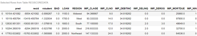
This creates a new file with the scored data that includes the 1788 rows from the validation data.

Print out the first five rows of the scored data to see the predicted value for LOAN for each row. Variable PRED holds this value. When we scored the data, we also calculated the residual value, and rstudent as columns in the data.

regscoredata=conn.CASTable("regscoredata", caslib="casuser")
regscoredata.head()

Use a selection method

To determine the most important variables and simplify our model, use the selection option to do a forward selection of the variables.

conn.regression.glm(
    table= dict(name = HomeEquity, where = '_PartInd_ = 1'),
    classVars=['IMP_REASON','IMP_JOB','REGION','BAD'],
    model={'depVar':'LOAN',
                   'effects':['IMP_REASON', 'IMP_JOB', 'REGION', 'BAD', 'IMP_CLAGE', 'IMP_CLNO',  
                    'IMP_DEBTINC', 'IMP_DELINQ', 'IMP_DEROG', 'IMP_MORTDUE', 'IMP_NINQ',
                    'IMP_VALUE', 'IMP_YOJ']
                  },
    selection={'method':'forward'}
)

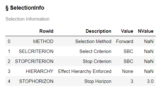
The forward selection method in linear regression is a step-by-step process of selecting the most relevant and significant variables to build the best possible model. It starts with adding one variable at a time and adds one by one until none of the remaining variables meet the proper criterion.

Below are the default selection criteria.

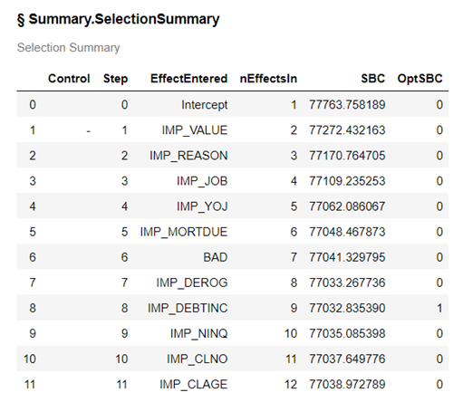
For this model 8 of our 14 variables were added to the model. The model selected is indicated by the 1 in the OptSBC column.

The analysis of variance table (ANOVA) indicates the overall statistics for the model.

The model fit statistics for the reduced model indicate the new smaller model is very similar in fit and accuracy as the full model.

Here is a complete listing of the included variables with the parameter estimates.

The Wrap-Up: Linear Regression

The GLM action in the regression action set for SAS Viya provides a powerful tool for performing linear regression. By carefully selecting and adding variables to our model, we can create accurate representations of real-world relationships and make informed decisions based on data analysis. Building a reliable model takes time and effort, but the results are worth it.

With the GLM Action and forward selection method, we can continue our imporoved understanding and prediction abilities, making linear regression in SAS a valuable tool for any data scientist or analyst.

In the next post, we will learn how fit a logistic regression.

Related Resources

SAS Help Center: Load a SASHDAT File from a Caslib
SAS Help Center: loadTable Action
Getting Started with Python Integration to SAS® Viya® - Part 5 - Loading Server-Side Files into Memory
SAS Help Center: Regression Action Set
SAS Help Center: glm Action
SAS Help Center: glmScore Action

Blogs