Fitting a Gradient Boosting Model - Learn how to fit a gradient boosting model and use your model to score new data

In Part 6, Part 7, and Part 9 of this series, we fit a logistic regression, decision tree and random forest model to the Home Equity data we saved in Part 4. In this post we will fit a gradient boosting model to the same data to predict who is likely to go delinquent on their home equity loan and we will score data with this model.

What is Gradient Boosting?

Gradient boosting is a powerful machine learning technique used for regression and classification tasks. It builds models in a sequential manner, where each new model tries to correct the errors made by the previous ones. The idea is simple: instead of building one complex model, gradient boosting combines several simple models—typically decision trees—into a strong one.

Here’s how it works in 5 easy steps:

Start with a simple decision tree: The process begins by training a small decision tree, which makes basic predictions. This tree is simple and might not capture all the complexities of the data, so it’s called a weak learner.

Identify the tree’s errors: Next, we calculate the difference between the tree’s predictions and the actual values. These differences represent the errors that the tree made.

Train a new tree to fix those errors: A new decision tree is then trained to predict the errors made by the first tree. This new tree focuses specifically on the data points that the first tree struggled with.

Add the new tree to the ensemble: The predictions from this second tree are combined with those of the first tree, improving the overall model. This process of adding trees continues, with each new tree aiming to correct the errors of the combined previous trees.

Combine all trees for final prediction: The final model is the sum of all the individual trees. Each tree contributes to the final prediction, resulting in a model that is much more accurate than any of the trees on their own.

By repeatedly adding decision trees that correct previous mistakes, gradient boosting builds a strong model capable of making precise predictions.

What is the Decision Tree Action Set?

The Decision Tree Action Set in SAS Viya offers a comprehensive suite of procedures and functions for building a variety of decision tree models. It includes actions for fitting decision trees, random forests, and gradient boosting models, among others. These tools enable users to create predictive models and explore the relationships between variables. The action set also includes options for model selection and scoring, providing users with the tools to interpret and validate their results effectively.

Load the Modeling Data into Memory

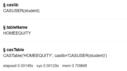
Let’s start by loading our data we saved in Part 4 into CAS memory. I will load the sashdat file for my example. Load the csv and parquet files using similar syntax.

conn.loadTable(path="homeequity_final.sashdat", caslib="casuser",
               casout={'name':'HomeEquity',
                               'caslib':'casuser', 'replace':True})

The home equity data is now loaded and ready for modeling.

Fit Gradient Boosting Model

Before fitting our Gradient Boosting Model in SAS Viya we need to load the decisionTree action set.

conn.loadActionSet('decisionTree')

The decisionTree action set contains several actions. Let’s display the actions to see what is available for use.

conn.help(actionSet='decisionTree')

This action set includes actions for both fitting and scoring decision trees, as well as for random forest and gradient boosting models. You can find examples of how to fit these models in Part 7 for Decision Trees and Part 9 for Random Forests.

Fit a gradient boosting model with the the gbtreeTrain action on the HomeEquity training data set (i.e. where _PartInd_=1). Save the model to a file named gb_model and to an astore format (more about this later in the post). Also specify the nominal columns in a list, assign seed the value of 1234, and set number of trees to fit to 1,000.

conn.decisionTree.gbtreeTrain(
    table    = dict(name = 'HomeEquity', where = '_PartInd_ = 1'),
    target   = "Bad", 
    inputs   = ['LOAN','IMP_REASON','IMP_JOB','REGION','IMP_CLAGE','IMP_CLNO',
                       'IMP_DEBTINC','IMP_DELINQ','IMP_DEROG','IMP_MORTDUE','IMP_NINQ',
                       'IMP_VALUE','IMP_YOJ'], 
    nominals = ['BAD','IMP_REASON','IMP_JOB','REGION'],
    nTree    = 1000,
    seed     = 1234,
    casOut   = dict(name = 'gb_model', replace = True),
    saveState= dict(name = 'gb_astore', replace = True)
)

Looking at the output we can see that 1000 trees were fit with average number of leaves at 15.6 each, along with all the additional model info.

Let’s take a look at the output tables currently in memory on the CAS Server

conn.table.tableInfo()

Score Validation Data

Now we will look at 2 ways to score data: Using the ASTORE file and using the Model file. There is a third method creating SAS Data Step score code using the gbtreeCode Action from the decisiontree action set that will not be shown here. You only need to score the data with one method so pick the one that works best for you.

Score Using the ASTORE File

First we will score the validation data using the ASTORE file (gb_astore). Using the head method you can see that the data is a binary representation.

conn.CASTable('gb_astore').head()

Before scoring the validation data using the ASTORE file in SAS Viya we need to load the aStore action set.

conn.loadActionSet('aStore')

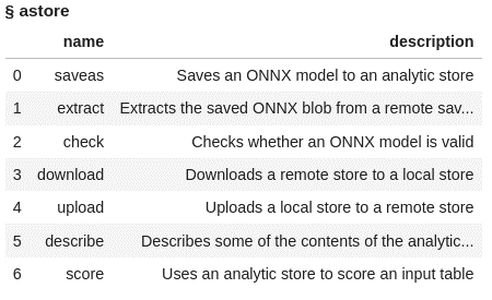
The actions included in the aStore actionset are listed below:

conn.builtins.help(actionSet='aStore')

Using the score action in the aStore action set score the validation data from the home equity data file. Use _PartInd_ = 0 to identify the validation rows from the data. Create a new data set with the scored values named gb_astore_scored.

conn.aStore.score(
    table    = dict(name = 'HomeEquity', where = '_PartInd_ = 0'),
    rstore = "gb_astore",
    out = dict(name="gb_astore_scored", replace=True),
    copyVars = 'BAD'
)

The new data has 1788 rows and 5 columns.

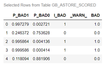
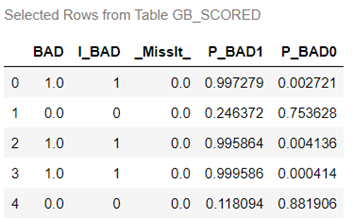
Use the head method to view the first 5 columns of gb_astore_scored file.

conn.CASTable('gb_astore_scored').head()

In this data file, you'll find five columns, each serving a distinct purpose:

P_BAD1: The predicted probability of an individual becoming delinquent on a home equity loan.
P_BAD0: The complement of P_BAD1 (1 - P_BAD1), representing the predicted probability of an individual not becoming delinquent on a home equity loan.
I_BAD: Here, you'll find the predicted classification value derived from the model.
_WARN_: Indicates why the model could not be applied because of things like missing values or invalid input values.
BAD: This column represents our target variable, acting as the label or dependent variable (Y).

Score Using the gb_model

For the second method lets score the validation data using in memory scoring table gb_model. First, use the head method to look at the first five rows of data. Here you can see we have rows that represent each column used in fitting the forest model.

conn.CASTable('gb_model').head()

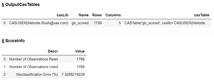
Now use gb_model and the gbtreeScore action in the decisionTree action set to score the validation data (_PartInd_ = 0). Create a scored data table called gb_scored.

conn.decisionTree.gbtreeScore(
    table    = dict(name = 'HomeEquity', where = '_PartInd_ = 0'),
    model = "gb_model",
    casout = dict(name="gb_scored",replace=True),
    copyVars = 'BAD',
    encodename = True,
    assessonerow = True
)

The data table gb_scored has 1788 rows and 5 columns. Output also includes the misclassification error at 7.33%

Use the head method to list the first 5 rows of gb_scored.

conn.CASTable('gb_scored').head()

In this data file, you'll find five columns, each serving a distinct purpose:

BAD: This column represents our target variable, acting as the label or dependent variable (Y).
I_BAD: Here, you'll find the predicted classification value derived from the model.
MissIt: A value of 0 indicates a correct prediction, while 1 signifies an incorrect prediction when the scored data aligns with the observed target value.
P_BAD1: The predicted probability of an individual becoming delinquent on a home equity loan.
P_BAD0: The complement of P_BAD1 (1 - P_BAD1), representing the predicted probability of an individual not becoming delinquent on a home equity loan.

Access Model

We’ll evaluate the fit of the gradient boosting model using the same metrics as with logistic regression, decision tree, and random forest models: confusion matrix, misclassification rates, and ROC plot. These metrics will help us gauge the model’s performance and later compare it to other models.

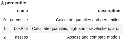
To compute these metrics, we’ll use the percentile action set along with the assess action. Start by loading the percentile action set and displaying the available actions.

conn.loadActionSet('percentile')
conn.builtins.help(actionSet='percentile')

We can use either of our scored data sets for doing assessment, as both have the same information and will give us the same output, so let’s use the gb_scored data created with the gb_model file above.

The access action creates two data sets named gb_assess and gb_assess_ROC.

conn.percentile.assess(
   table = "gb_scored",
   inputs = 'P_BAD1',
   casout = dict(name="gb_assess", replace=True),
   response = 'BAD',
   event = "1"
)

Using the fetch action list the first 5 rows of the gb_assess dataset for inspection. You can see the values at each of the depths of data from 5% incremented by 5.

display(conn.table.fetch(table='gb_assess', to=5))

Using the fetch action again on the gb_assess_ROC data, take a look at the first 5 rows. Here if we select cutoff of .03 the predicted true positives for our validation data would be 334 and true negatives 1211. Typically, the default cutoff value is .5 or 50%.

conn.table.fetch(table='gb_assess_ROC', to=5)

Let’s bring the output data tables to the client as data frames to calculate the confusion matrix, misclassification rate, and ROC plot for the forest model.

gb_assess = conn.CASTable(name = "gb_assess").to_frame()
gb_assess_ROC = conn.CASTable(name = "gb_assess_ROC").to_frame()

Confusion Matrix

The confusion matrix can be quickly calculated using the columns generated in the gb_assess_ROC file.

This matrix compares the predicted values with the actual values, providing a detailed breakdown of true positives, true negatives, false positives, and false negatives.

These metrics allow us to evaluate the model’s performance and assess its accuracy in predicting the target outcome.

For this analysis, use a cutoff value of 0.5. This means that if the predicted probability is 0.5 or higher, the model predicts delinquency on a home equity loan. If the predicted probability is less than 0.5, the model predicts no delinquency.

cutoff_index = round(gb_assess_ROC['_Cutoff_'],2)==0.5
conf_mat = gb_assess_ROC[cutoff_index].reset_index(drop=True)
conf_mat[['_TP_','_FP_','_FN_','_TN_']]

At the 0.5 cutoff value the true positives are 273 and the true negatives are 1384.

Misclassification Rate

We can easily calculate the misclassification rate using the columns generated for the confusion matrix, which shows how frequently the model makes incorrect predictions.

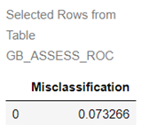
conf_mat['Misclassification'] = 1-conf_mat['_ACC_']
miss = conf_mat[round(conf_mat['_Cutoff_'],2)==0.5][['Misclassification']]
miss

The misclassification rate of 7.3% matches the result obtained when we applied the gb_model to score the validation data.

ROC Plot

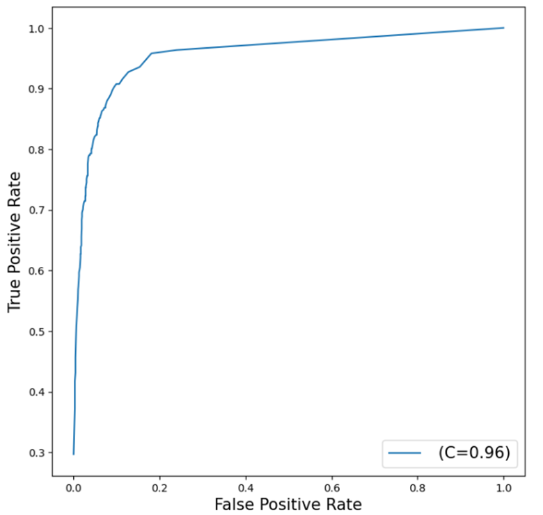
Our final assessment metric will be a ROC (Receiver Operating Characteristic) Chart, which visualizes the trade-off between sensitivity and specificity. This chart offers a comprehensive view of the forest model's performance, where a curve closer to the top left corner indicates a more effective model.

To plot the ROC Curve, use the matplotlib package in Python.

from matplotlib import pyplot as plt
 
plt.figure(figsize=(8,8))
plt.plot()
 
plt.plot(gb_assess_ROC['_FPR_'],gb_assess_ROC['_Sensitivity_'], label=' (C=%0.2f)'%gb_assess_ROC['_C_'].mean())
 
plt.xlabel('False Positive Rate', fontsize=15)
plt.ylabel('True Positive Rate', fontsize=15)
plt.legend(loc='lower right', fontsize=15)
plt.show()

The curve generated by the gradient boosting model is fairly close to the top left corner, indicating that the model fits the data reasonably well, though there’s still room for improvement.

The AUC (Area Under the Curve) value of 0.96 is another indicator of the model’s fit. This suggests that our gradient boosting model performs better than a random classifier, which has an AUC of 0.5, but it doesn’t reach the ideal scenario of an AUC of 1, which would represent a perfect model.

The Wrap-Up: Fitting a Random Forest Model

Fitting a gradient boosting model is straightforward using the decisionTree action set, particularly with the gbtreeTrain action, which streamlines the model creation process. Similarly, the gbtreeScore action allows for efficient scoring of holdout or new data, making it easy to evaluate the model's overall effectiveness.

In the next post, we will explore fitting a neural network model to our dataset.

Related Resources

SAS Help Center: Decision Tree Action Set
SAS Help Center: gbtreeTrain Action
SAS Help Center: gbtreeScore Action
SAS Help Center: gbtreeCode Action
SAS Help Center: assess Action
Getting Started with Python Integration to SAS® Viya® - Part 5 - Loading Server-Side Files into Memory

Blogs