My second post in Graphically Speaking described modifying dynamic variables in ODS Graphics. Little did I know the extent to which it would launch a series of blogs, papers, conference presentations, and even a book chapter. It was my initial foray into the area that I like to call "Highly Customized Graphs," which is a set of techniques that enables you to modify all of the components of the graphs that analytical procedures produce: the data object, graph template, and the dynamic variables. This technique even enables you to add SG annotation (although we won't get into that here). Before we take a deeper dive into data, documents, and dynamics, here are sources of more information about highly customized graphs.
Fit Plot Customizations
Advanced ODS Graphics Examples
Advanced ODS Graphics: Annotating multiple panels
Advanced ODS Graphics: Annotating graphs from analytical PROCs
Advanced ODS Graphics: Modifying Dynamic Variables in ODS Graphics
Highly Customized Graphs Using ODS Graphics
Annotating Graphs from Analytical Procedures
If you are not familiar with the techniques for highly customized graphs in my previous articles, you should review them before proceeding. You might want to start with Rick Wicklin's article, A SAS programming technique to modify ODS templates. This article was prompted when a user in SAS Communities asked about modifying the biplot that PROC PRINQUAL produces. To answer it, I first tried a trick from Fit Plot Customizations. I added an ID variable to the input data set, specified it in the PROC PRINQUAL step, and modified the template to use that ID variable to change an aspect of the graph. I got a warning:
WARNING: The variable (IDLAB2) cannot be found in the data model. The likely
         cause is that the variables used in the same plot statement have
different observation counts. The generated graph may be incorrect. |
This had me scratching my head at first. I constructed my ID variable so that it had precisely the same number of observations as the other variables in the vector plot, so how could this be? Here is where the ODS document comes in handy. You can use an ODS document to capture the graph including the dynamic variables, and you can use PROC DOCUMENT to display them. First, here is a brief refresher course about dynamic variables using examples from more familiar procedures such as PROC REG and PROC GLM. Dynamic variables are name and value pairs. They provide all of the information that is needed to create a graph or a table that is not data and also cannot be known until the procedure is actually run. If the graph title is "Fit Plot for Height" (where Height is a variable name), then "Fit Plot for" is known at the time the procedure is written, but the variable name, Height, can only be known when the the procedure is run. When the table of statistics in a PROC REG fit plot says "Observations" and "19", then "19" can only be known at the time the procedure is run. The other strings might appear in the template or come in through dynamic values. It will largely depend on the different purposes for which the template is used.
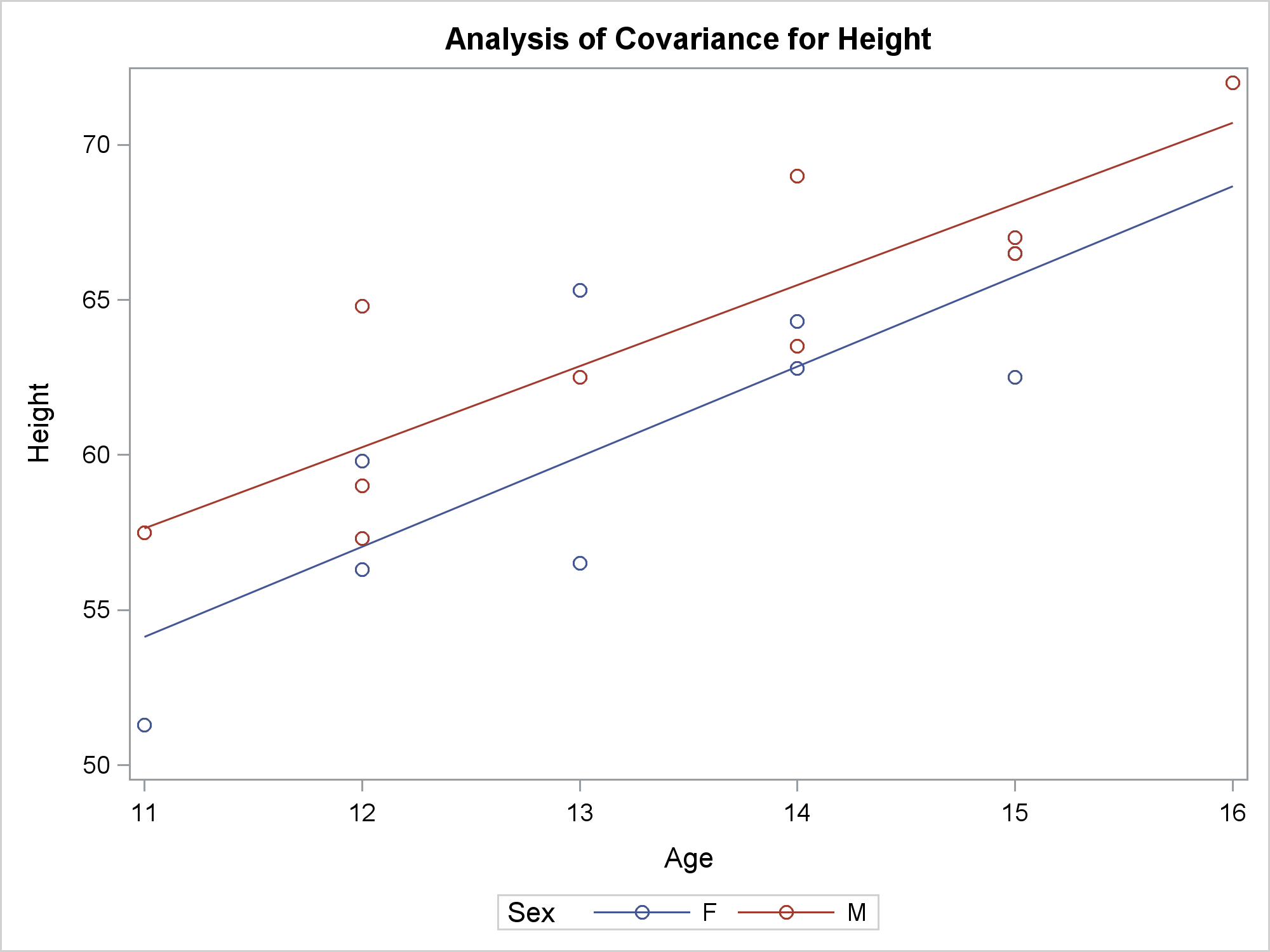
The following steps create an ODS document and capture the results from PROC REG and PROC GLM. The PROC REG step fits a simple regression model, and the PROC GLM step fits an analysis of covariance model that fits a separate line (separate slope and intercept) for each gender. Both steps use an ODS OUTPUT statement create a SAS data set from the data objects that underlies the graph, which are printed by PROC PRINT.
ods graphics on; ods document name=MyDoc (write); proc reg data=sashelp.class; model height = age; ods output fitplot=ap; quit; proc print; run; proc glm data=sashelp.class; class sex; model height = age | sex; ods output ancovaplot=ap; quit; proc print; run; ods document close; |
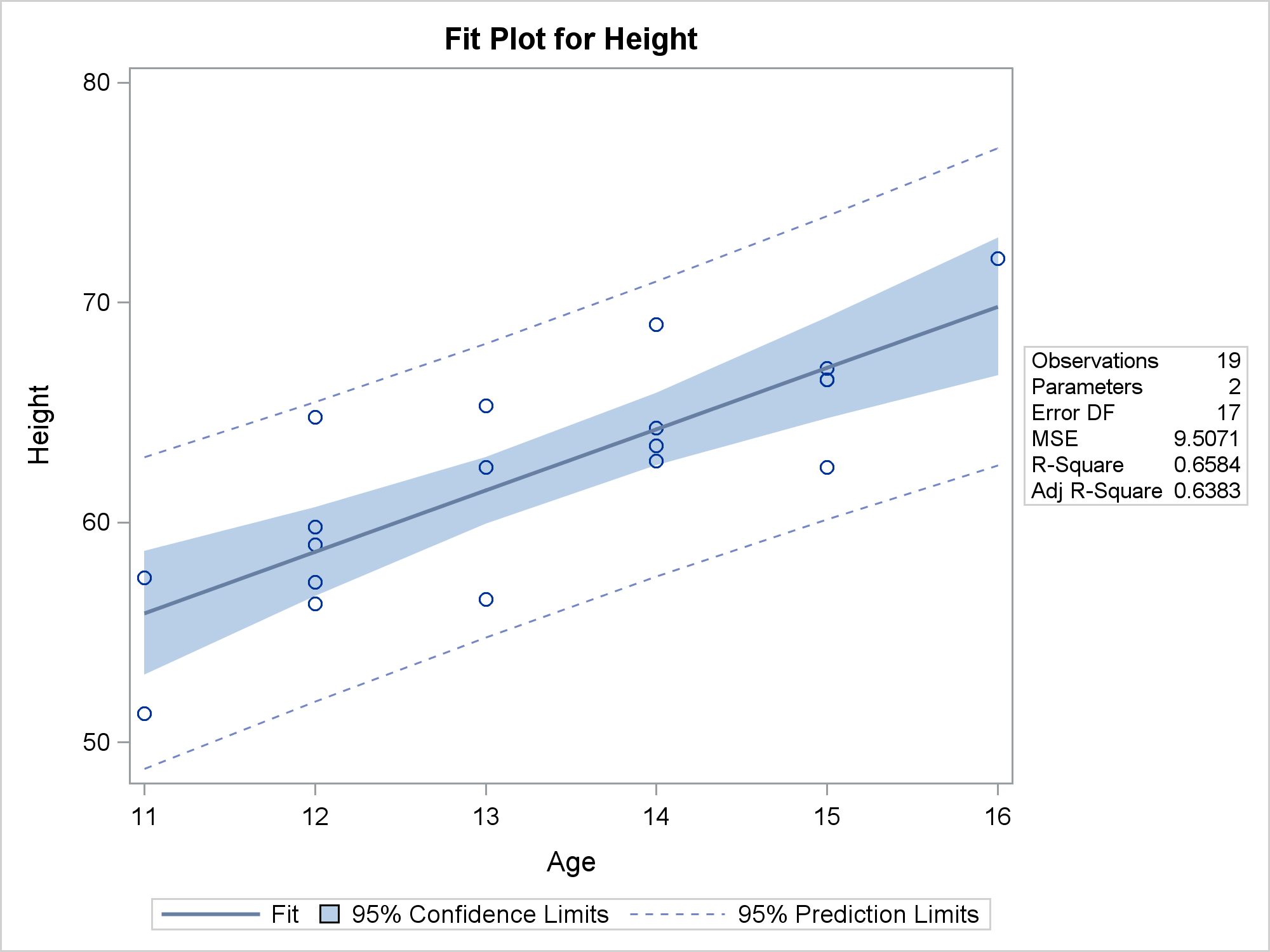
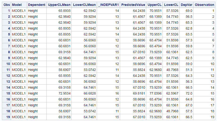
The data set made from the PROC REG data object is quite straight-forward and is displayed next. It has 19 observations (which match the number of observations in the input data set) some ID columns (which identify the model and the dependent variable, but are not used in the graph), and columns for the information that is plotted: X and Y coordinates for the scatter plot, fit function, and confidence and prediction limits.
The PROC GLM data object is different. It has three sets of columns. The first set contains a variable ID column (Dependent), which is also in the PROC REG data object. This column identifies the output data set observations when there are multiple dependent variables. The second set contains scatter plot columns (_X7 through _YVAR), The third set defines the two lines for the two genders. The scatter plot columns have two partitions. First there are two observations, one for each level of the CLASS variable (Sex). This ensures that the first group corresponds to the first CLASS level ('F' sorts ahead of 'M') and the second group corresponds to the second CLASS level. This ensures consistency in the graph if the data are sorted or if there is a BY variable. Other columns have missing values ensuring that those values do not get used in the graph. While there are other ways to accomplish this besides prepending the data object with extra rows, that was not the case when much of the SAS/STAT ODS Graphics code was written. The line columns have four observations, two for each gender, that provide the starting and ending point for each line. The remaining observations are missing. There is no correspondence between the rows in the the scatter plot set and the rows in the lines set.
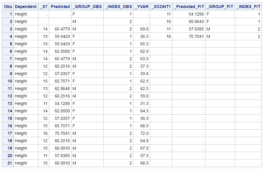
Notice in both data objects that our input data set variable names, Sex, Height, and Age do not appear as data object column names. This is deliberate. The procedure writer must take full control over the column names. If the procedure used some of your names and created other names, things will implode when a name from each set happens to match. When I helped with the SAS Communities question, I added a variable Group to the data set, and I needed to work with the column name IDLAB2 when I modified the template to use it. The procedure (quite correctly) renamed it. Also notice that we do not require that the data set made from a graph data object be beautiful or well suited for input to another procedure or well suited for any purpose other than the purpose for which it was intended: making the graph.
We can use PROC DOCUMENT to examine the dynamic variables. First, we need to list the contents of the document.
proc document name=MyDoc; list / levels=all; quit; |
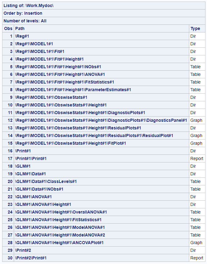
The output gives us the paths of all of the tables and graphs that are in the document. You can copy and paste the paths into OBDYNAM statements for use with PROC DOCUMENT. I find that I can never anticipate the names; I always need to list the contents of the ODS document.
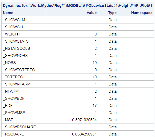
proc document name=MyDoc; obdynam \Reg#1\MODEL1#1\ObswiseStats#1\Height#1\FitPlot#1; obdynam \GLM#1\ANOVA#1\Height#1\ANCOVAPlot#1; quit; |
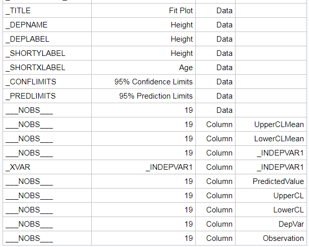
The list of dynamic variables from PROC REG is long--only the beginning and end are displayed below. This is because PROC REG displays a number of statistics by default, many more by request, and it does so in a flexible way. Dynamic variable names that contain SHOW are binary: 1 means the corresponding statistic is displayed, and 0 means it is not displayed. A corresponding dynamic variable contains the value of the statistic even if it is not displayed. This gives you incredible power for post hoc customization. Notice that some of the dynamic values are Type='Data' and others are Type='Column'. A procedure can create a dynamic variable in the process of creating the graph (Type='Data') or in the process of creating a data object column that goes into making a graph. ODS Graphics makes its own dynamic variables too. They begin and end with three underscores. ___NOBS___ appears on each of the columns, and it shows that each column has 19 observations.
The list of dynamic variables for PROC GLM is shorter, since the PROC GLM analysis of covariance plot does not display any of the statistics that PROC REG displays in its fit plot. Notice the ___NOBS___ variables. They have two different values: 21 and 4.
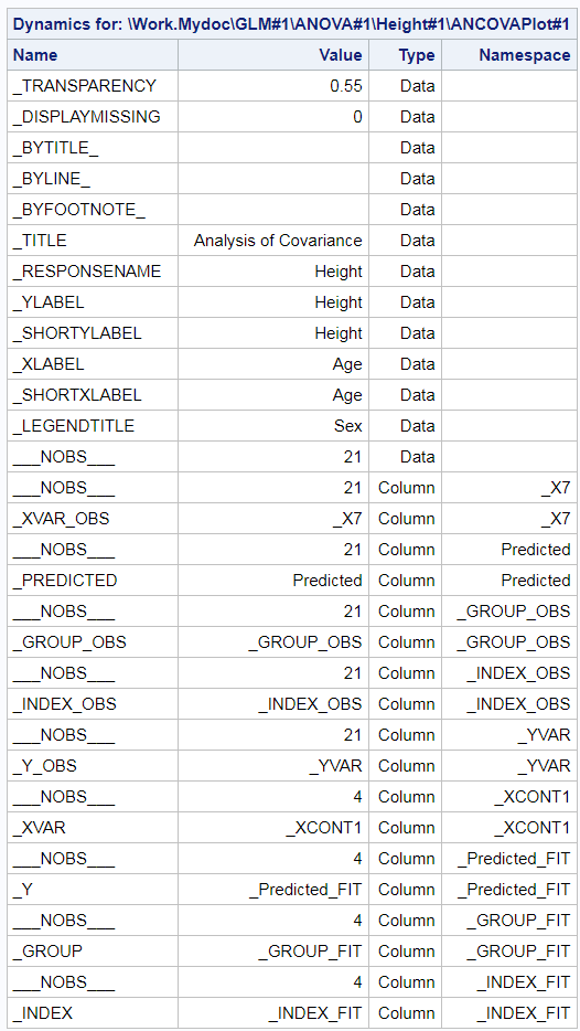
You can be a sophisticated user of ODS Graphics and never need to know this, but the list of dynamic variables shows you that the ANCOVA graph output data set is made from two data objects: one with 21 observations and one with 4. This is consistent with the data object. Much like a DATA step with a MERGE statement, the two sets of columns are created next to each other and the one with fewer observations is padded with missing values. The procedure writer has a good bit of discretion in how it sets up data object(s). He could have created one data object and used it. Instead, he created two data objects and then told ODS Graphics to combine them to create the input for the graph. This latter approach is quite common when a graph is created from two quite different overlaid parts. I use two data objects in my vector plots (preference mapping in PROC TRANSREG and multidimensional preference analysis or MDPREF in PROC PRINQUAL). Both consist of a scatter plot (data object one) that has an overlaid vector plot (data object two). Both data objects are different sizes, and there is no correspondence between the rows, so it is easier for the PROC writer to create two data objects.
When I answered the question about modifying the vectors and vector labels in the PROC PRINQUAL MDPREF plot, I first tried a trick. I created a new input variable and specified it in the ID statement. This put it into the scatter plot data object. Then I tried to use it in the vector plot to change the colors of the vectors and vector labels. Since most of my variables in the VECTORPLOT statement came from the second data object and one came from the first, I got the warning.
WARNING: The variable (IDLAB2) cannot be found in the data model. The likely
         cause is that the variables used in the same plot statement have
different observation counts. The generated graph may be incorrect. |
If you get this warning, interpret it as an error. As the message warned, my group variable appeared to have an effect, but my graph was incorrect. ODS Graphics does this to protect us from ourselves. It will almost never make sense to create a plot using variables from multiple data objects (or in the words of the message, "data models") in a single statement.
Now let's look at the answer that I gave to the SAS Communities question. The user wants to change the colors of groups of vectors and vector labels in the plot. This is actually a hard problem. To do this, I need to modify the data object to add a group variable. Then I need to modify the graph template to use the group variable. If the PROC PRINQUAL graph were like the regression fit plot in my Fit Plot Customizations blog, that would be all I would have to do. Since the PROC PRINQUAL graph is constructed from two data objects, there is more work. ODS Graphics will not simultaneously use columns from two data objects in a single statement. However, I can trick it. Following the examples in my sources listed above, I can output the data objects to a data set, capture the dynamic variables in an ODS document, and output them to a data set. Then I can use a DATA step and CALL EXECUTE to reconstruct the graph outside of PROC PRINQUAL and have it use the group variable to change the colors.
* Ensure we are not using the modified template (if we run this more than once).
  OK if you get a warning the first time that it does not exist.;
proc template;
   delete Stat.Prinqual.Graphics.MDPref /  store=work.modtemp;
quit;

* Default analysis;
proc prinqual data=cars mdpref;
   ods output mdprefplot=m;
   transform ide(mpg -- cargo);
   id model;
run;

* Default data object;
proc print data=m; run;

* Store template in a file.  Look at it.;
proc template;
   source Stat.Prinqual.Graphics.MDPref / file='tpl.tpl' store=sashelp.tmplstat;
quit;

* Store modified template in WORK so it disappears when SAS closes.;
ods path (prepend) work.modtemp(update);
* Don't have to show it, but it is nice to see that it worked.;
ods path show;

* Modify template.  You cannot write code like this in a vacuum.
  You must look at the original template.;
data _null_;
   infile 'tpl.tpl' end=eof;
   input;
   * Add proc call;
   if _n_ = 1 then call execute('proc template;');
   * Remove Store option;
   i = index(lowcase(_infile_), '/ store = ');
   if i then substr(_infile_, i) = ';';
   * Skip using the group variable as an ID variable.;
   _infile_ = tranwrd(_infile_, '_id2=IDLAB2', ' ');
   _infile_ = tranwrd(_infile_, ' _id2 ', ' ');
   * Find start of vectorplot.;
   v + index(lowcase(_infile_), 'vectorplot');
   if v then do;
      * Add group var.;
      _infile_ = tranwrd(_infile_, '/', '/ group=idlab2');
      * Remove current label attributes.;
      _infile_ = tranwrd(_infile_, 'datalabelattrs', 'primary=true; *');
      * Flag end of vectorplot statement.;
      if index(_infile_, ';') then v = 0;
   end;
   * Write out line (original or modified).;
   call execute(_infile_);
   * End the PROC call.;
   if eof then call execute('run;');
run;

* Let's see what we did.;
proc template;
   source Stat.Prinqual.Graphics.MDPref;
quit;

* Map the variable names to group numbers.
  You don't necessarily need to make an informat.
  That just seemed to be an easy way to specify groups of variables
  that will have the same colors.;
data cntlin;
   length start $ 24;
   Type    = 'i';
   FmtName = "CarFmt";
   input start $ label;
   datalines;
MPG           1
Acceleration  1
Reliability   2
Braking       3
Handling      3
Ride          3
Visibility    4
Comfort       4
Quiet         4
Cargo         5
;

proc format cntlin=cntlin; quit;

* Add a new group variable.  Make it reflect the color groups that you want.
  It will become idlab2 (the second ID variable) in the data object;
data cars2;
   set cars;
   array __x[*] _numeric_;
   * Here is where you will substitute your logic for making the group
     names if you want some other grouping. I am using my informat.;
   if _n_ le 10 then group = input(vname(__x[_n_]), carfmt.);
run;

* Need the ODS Document to access the dynamics.;
ods document name=MyDoc (write);
* Add group as an ID variable.  Use the modified data set and template.
  We will ignore this graph, but it will provide the pieces that we need
  for the real graph.;
proc prinqual data=cars2 mdpref;
   ods output mdprefplot=m;
   transform ide(mpg -- cargo);
   id model group;
run;
* The warning is because of I am using two data objects in one statement.
  ODS Graphics does not accept variables from different data objects
  (although in some ways it appears that it does).
  I need one more major step, then I can create the graph outside PRINQUAL.;
ods document close;

* Need to see the path for the graph.;
proc document name=MyDoc;
   list / levels=all;
quit;

* Display and store the dynamics in a SAS data set.;
proc document name=MyDoc;
   ods output dynamics=dynamics;
   obdynam \Prinqual#1\MDPREF#1\MDPrefPlot#1;
quit;

* Examine the new data object just to better see what is going on.;
proc print data=m; run;

* This calls SGRENDER using the modified template and populates the
  DYNAMIC statement with all of the dynamic name/value pairs.;
 data _null_;
   * Skip the number of observations variables.
     They are not needed for our purposes.
     Now ODS Graphics will no longer know that there are two data objects.;
   set dynamics(where=(label1 ne '___NOBS___')) end=eof;
   * Call PROC SGRENDER, start writing a DYNAMIC statement.;
   if _n_ = 1 then do;
      call execute('proc sgrender data=m ' ||
                   'template=Stat.Prinqual.Graphics.MDPref;');
      call execute('dynamic');
   end;
   * Populate the DYNAMIC statement with name value pairs.
     Use formatted numeric values or quoted character values.;
   if cvalue1 ne ' ' then
      call execute(catx(' ', label1, '=',
                   ifc(n(nvalue1), cvalue1, quote(trim(cvalue1)))));
   * Wrap things up with a RUN statement.;
   if eof then call execute('; run;');
run;

* Unfortunately this problem requires *all* of the
  steps for making highly customized graphs.
  1) Modify the template.
  2) Output the data object.  I modified it by using an ID variable before hand,
     (just because that was how I started approaching this)
     but I could have modified it after the fact.
  3) Access the dynamic variables.
  4) Use CALL EXECUTE to make SGRENDER code that uses the data object,
modified template, and dynamic variables.; |
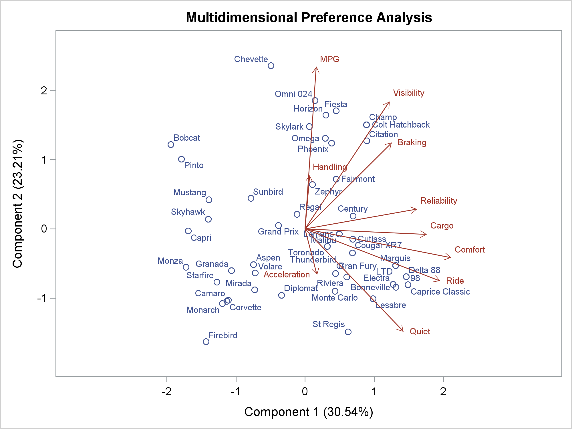
Here is the original graph, which uses GraphData1 for the scatter plot and GraphData2 for the vector plot.
Here is the customized graph.
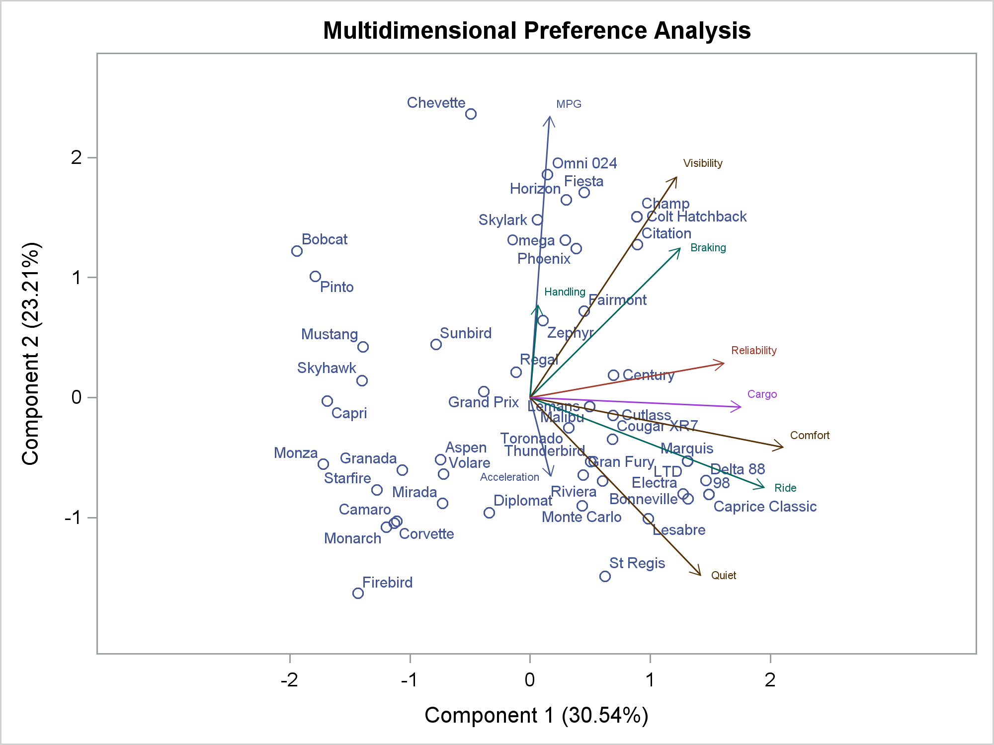
Now we see the specified grouping. MPG and Acceleration use GraphData1 (blue), Reliability uses GraphData2 (red), Braking, Handling, and Ride use GraphData3 (green), and so on. You could create a discrete attribute map if you wanted more explicit control over the colors. If you are interested in this type of graph, also see vector plots and adjusting point labels for a way to print short vectors.
Many graph customizations are simple. This one is more involved. Yes, there is a learning curve, but when you break things down, none of the steps is hard. The template modification step uses functions like TRANWRD to modify templates. You could choose to use an editor, but the DATA step gives you a reproducible chain of steps that creates the graph. The final DATA step that uses CALL EXECUTE might be a bit harder to understand. Much like the macro language, it uses a program to write a program. In this case, it is writing a PROC SGRENDER step that only consists of three statements.
Of course, everything you might want to do is not available by simply flipping an option. ODS Graphics gives you incredible flexibility to create highly customized graphs if you are willing to do a bit of programming. Most of the time you can get by without understanding all of the intricacies of data objects and dynamic variables, but some advanced customizations require a deeper dive.
