Fit Plot Customizations

A customer wants to use PROC REG to fit a simple regression model but display in the fit plot markers that differentiate groups of individuals.

Click on a graph to enlarge.

Before we see how to do that, let's look at some simpler examples.

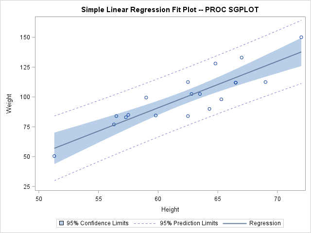
The following step fits a linear regression model and displays an ordinary fit plot:

proc sgplot data=sashelp.class;
   title 'Simple Linear Regression Fit Plot -- PROC SGPLOT';
   reg y=weight x=height / cli clm;
run;

The CLI option produces prediction limits and the CLM option produces confidence limits.

The following steps fit the same model, but males are displayed as filled squares and females are displayed as filled circles:

ods graphics on / attrpriority=none;
 
proc format;
   value $sex 'M' = 'Male' 'F' = 'Female';
run;
 
proc sgplot data=sashelp.class;
   title 'Simple Regression but with a Classification Variable Displayed -- PROC SGPLOT';
   styleattrs datasymbols=(squarefilled circlefilled);
   reg y=weight x=height / cli clm nomarkers;
   scatter y=weight x=height / group=sex  name='scatter';
   keylegend 'scatter' / location=inside across=1 position=topleft;
   format sex $sex.;
run;

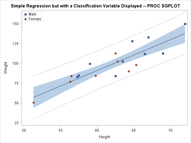
These examples all use the HTMLBlue style, which is an ATTRPRIORITY=COLOR style. The ATTRPRIORITY=NONE option enables marker differences to be displayed as well as color differences. The $SEX format provides meaningful labels in the legend. The STYLEATTRS statement creates the custom markers. The NOMARKERS option suppresses the markers from being displayed by the REG statement. Instead, they are displayed by the SCATTER statement, which uses the GROUP=SEX option to distinguish the groups. The KEYLEGEND statement displays a legend inside the graph.

While this is a nice graph and it is easy to make, the customer specifically wanted PROC REG, because PROC REG displays a table of statistics along with the fit plot. The following step illustrates:

proc reg data=sashelp.class;
   model  weight = height;
quit;

PROC REG will not use the classification variable SEX in the graph without a template change. However before you can proceed, you need to see if the SEX variable is available in the data object that underlies the graph. The following step outputs the data object to a SAS data set:

proc reg data=sashelp.class;
   ods select fitplot;
   ods output fitplot=fp;
   model weight = height;
   id sex;
quit;

If you print the data set, you will see that the SEX variable is in the output data set, but it is named ID1. In fact, not one of the original variable names is present in the output data set. This is because analytical procedures need to have precise control the data object column names so that the templates will work with the wide variety of models that people specify.

We will use a DATA step and CALL EXECUTE to modify the graph template for the fit plot. There are other ways to modify a template, but the DATA step provides a parsimonious way to show small changes to large templates. You cannot write template modification code like the DATA step below without first looking at the template. The following step writes the fit plot template to a file called temp.tmp:

proc template;
   source Stat.REG.Graphics.Fit / file='temp.tmp';
quit;

The following step reads the template, adds a PROC TEMPLATE statement, drops the MARKERATTRS= option from the SCATTERPLOT statement, and adds the GROUP=ID1 option. It also adds options to the BEGINGRAPH statment to control the markers:

options source;
data _null_;
   infile 'temp.tmp';
   input;
   if _n_ = 1 then call execute('proc template;');
   if left(_infile_) =: 'SCATTERPLOT y=DEPVAR' then do;
      _infile_ = tranwrd(_infile_, 'markerattrs=GRAPHDATADEFAULT', ' ');
      _infile_ = tranwrd(_infile_, '/', '/ group=id1 ');
      end;
   if left(_infile_) =: 'BeginGraph' then
      _infile_ = 'BeginGraph / attrpriority=none' ||
                 ' datasymbols=(squarefilled circlefilled);';
   call execute(_infile_);
run;

Other statements are executed as is. The OPTIONS SOURCE statement is not required. It shows the code that is generated by CALL EXECUTE, so it can help you understand what is happening when things do not work.

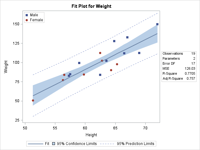
The following step uses the modified template:

proc reg data=sashelp.class;
   ods select fitplot;
   model weight=height;
   id sex;
quit;

You can also add a NAME= option to the SCATTERPLOT statement and a DISCRETETELEGEND statement after the SCATTERPLOT statement to display the values of SEX in a legend:

data _null_;
   infile 'temp.tmp';
   input;
   if _n_ = 1 then call execute('proc template;');
   if left(_infile_) =: 'SCATTERPLOT y=DEPVAR' then do;
      _infile_ = tranwrd(_infile_, 'markerattrs=GRAPHDATADEFAULT', ' ');
      _infile_ = tranwrd(_infile_, '/', '/ group=id1 name="sc"');
      end;
   if left(_infile_) =: 'BeginGraph' then
      _infile_ = 'BeginGraph / attrpriority=none' ||
                 ' datasymbols=(squarefilled circlefilled);';
   call execute(_infile_);
   if left(_infile_) =: 'SCATTERPLOT y=DEPVAR' then
   call execute('discretelegend "sc" / location=inside across=1 autoalign=(topleft);');
run;
 
proc reg data=sashelp.class;
   ods select fitplot;
   model weight=height;
   id sex;
   format sex $sex.;
quit;

The DATA _NULL_ step reads the same (unmodified) temp.tmp file and creates a new template modification.

The following step deletes the modified template:

proc template;
   delete Stat.REG.Graphics.Fit / store=sasuser.templat;
quit;

This all works because the SEX variable appears in the data object when it is specified in the ID statement. It appears in the data object so that it can appear in HTML tooltips. What if it had not been there? The next part of the example shows how you can output the data object, modify it (that is, merge in the SEX variable), and create the desired graph with PROC SGRENDER. The PROC SGRENDER step uses the modified data object, the modified graph template, and the style template, but it needs one more thing: dynamic variables. Procedures set dynamic variables that control many aspects of the graphs and contain other values such as the statistics that are displayed in the table.

The following step captures the graph, including the dynamic variables and their values, in an ODS document. It also captures the data object in a SAS data set:

ods document name=MyDoc (write);
proc reg data=sashelp.class;
   title 'Not Shown';
   ods select fitplot;
   ods output fitplot=fp;
   model weight=height;
quit;
ods document close;

The following step lists the contents of the ODS document:

proc document name=MyDoc;
   list / levels=all;
quit;

You need to copy the path of the graph from the LIST statement output into the OBDYNAM statement.

The following step creates a SAS data set that contains the values of the dynamic variables:

proc document name=MyDoc;
   ods exclude dynamics;
   ods output dynamics=dynamics;
   obdynam \Reg#1\MODEL1#1\ObswiseStats#1\Weight#1\FitPlot#1;
quit;

The following step displays the data set of dynamic variables (some of which are shown):

proc print; 
run;

The following step merges the SEX variable into the output data set made from the data object:

data both(drop=height weight rename=(sex=id1));
   merge sashelp.class(keep=height weight sex) fp;
   if height ne _indepvar1 or weight ne depvar then put _all_;
   format sex $sex.;
run;

The SEX variable is renamed ID1 so that it can work with the same template as before. You cannot rely on a merge operation being as simple as the one shown here. Data sets made from graph data objects can vary from input data sets in many ways. An IF statement is added to check the merge only to emphasize that you need to carefully combine data from separate sources and always check your results.

The following step modifies the template (as before):

data _null_;
   infile 'temp.tmp';
   input;
   if _n_ = 1 then call execute('proc template;');
   if left(_infile_) =: 'SCATTERPLOT y=DEPVAR' then do;
      _infile_ = tranwrd(_infile_, 'markerattrs=GRAPHDATADEFAULT', ' ');
      _infile_ = tranwrd(_infile_, '/', '/ group=id1 name="sc"');
      end;
   if left(_infile_) =: 'BeginGraph' then
      _infile_ = 'BeginGraph / attrpriority=none' ||
                 ' datasymbols=(squarefilled circlefilled);';
   call execute(_infile_);
   if left(_infile_) =: 'SCATTERPLOT y=DEPVAR' then
   call execute('discretelegend "sc" / location=inside across=1 autoalign=(topleft);');
run;

The following step uses CALL EXECUTE to run PROC SGRENDER along with a DYNAMIC statement that provides the value of each of the dynamic variables:

data _null_;
   set dynamics(where=(label1 ne '___NOBS___')) end=eof;
   if nmiss(nvalue1) and cvalue1 = '.' then cvalue1 = ' ';
   if _n_ = 1 then do;
      call execute('proc sgrender data=both');
      call execute('template=Stat.REG.Graphics.Fit;');
      call execute('dynamic');
   end;
   if cvalue1 ne ' ' then
      call execute(catx(' ', label1, '=',
                   ifc(n(nvalue1), cvalue1, quote(trim(cvalue1)))));
   if eof then call execute('; run;');
run;

The DATA _NULL_ step with the CALL EXECUTE statements generate the following DYNAMIC statement:

dynamic _SHOWCLM = 1 _SHOWCLI = 1 _WEIGHT = 0 _SHOWSTATS = 1 _NSTATSCOLS = 2
   _SHOWNOBS = 1 _NOBS = 19 _SHOWTOTFREQ = 0 _TOTFREQ = 19 _SHOWNPARM = 1 
   _NPARM = 2 _SHOWEDF = 1 _EDF = 17 _SHOWMSE = 1 _MSE = 126.02868962 
   _SHOWRSQUARE = 1 _RSQUARE = 0.7705068427 _SHOWADJRSQ = 1 
   _ADJRSQ = 0.7570072452 _SHOWSSE = 0 _SSE = 2142.4877235 _SHOWDEPMEAN = 0
   _DEPMEAN = 100.02631579 _SHOWCV = 0 _CV = 11.223296526 _SHOWAIC = 0 
   _AIC = 93.780394884 _SHOWBIC = 0 _BIC = 96.223301459 _SHOWCP = 0 _CP = 2
   _SHOWGMSEP = 0 _GMSEP = 140.9531397 _SHOWJP = 0 _JP = 139.29486747 
   _SHOWPC = 0 _PC = 0.2834915472 _SHOWSBC = 0 _SBC = 95.669272843 _SHOWSP = 0 
   _SP = 7.876793101 _TITLE = "Fit Plot" _DEPNAME = "Weight" _DEPLABEL = "Weight"
   _SHORTYLABEL = "Weight" _SHORTXLABEL = "Height" _CONFLIMITS = "95% Confidence
   Limits" _PREDLIMITS = "95% Prediction Limits" _XVAR = "_INDEPVAR1";

The following step deletes the modified template:

proc template;
   delete Stat.REG.Graphics.Fit / store=sasuser.templat;
quit;

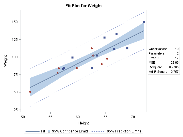
You can process the data set of dynamic variables and create a similar graph using PROC SGPLOT:

data _null_;
   length s $ 500;
   retain s;
   set dynamics(keep=label1 nvalue1) end=eof;
   if label1 = '_NOBS'    then l = 'Observations';
   if label1 = '_NPARM'   then l = 'Parameters';
   if label1 = '_EDF'     then l = 'Error DF';
   if label1 = '_MSE'     then l = 'MSE';
   if label1 = '_RSQUARE' then l = 'R-Square';
   if label1 = '_ADJRSQ'  then l = 'Adj R-Square';
   if l ne ' ' then s = catx(' ', s, quote(l), '=', quote(put(nvalue1, best6.)));
   if eof then call symputx('insets', s);
run;
 
%put &insets;
 
proc sgplot data=sashelp.class;
   title 'PROC SGPLOT with an Inset Table';
   styleattrs datasymbols=(squarefilled circlefilled);
   reg y=weight x=height / cli clm nomarkers;
   scatter y=weight x=height / group=sex  name='scatter';
   keylegend 'scatter' / location=inside across=1 position=topleft;
   inset (&insets) / position=bottomright border;
   format sex $sex.;
run;

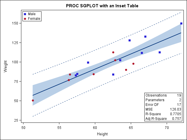
The DATA step generates the following list of insets:

"Observations" = "    19" "Parameters  " = "     2" "Error DF    " = "    17" 
"MSE         " = "126.03" "R-Square    " = "0.7705" "Adj R-Square" = " 0.757"

ODS Graphics provides you with ways to make simple graphs and customize every aspect of them. While not shown in this example, you can also annotate graphs and modify dynamic variables. For more information about SG annotation and the techniques shown in this blog, see the free book Advanced ODS Graphics Examples