A vector plot draws a line (potentially ending in an arrowhead) from one point in a graph to another point. Often, that first point is the origin (0,0) although both PROC SGPLOT and the GTL enable you to specify other points. In this post, I will show you how to pick a different origin: that is, how to pick a point on a line that is a specified distance from the end point. This creates short vectors and a cleaner look than the traditional long vectors. I also show how to modify the positions of the vector labels.

I use vector plots in two of my procedures: TRANSREG for preference mapping (PREFMAP) and PRINQUAL for multidimensional preference analysis (MDPREF). In this example, I only illustrate MDPREF, which provides a simultaneous display of the rows and columns of a data matrix. For more information, see PROC PRINQUAL documentation.

Click to see the data.

ods graphics on;
proc prinqual data=cars mdpref;
   ods output mdprefplot=m;
   transform ide(mpg -- cargo);
   id model;
run;

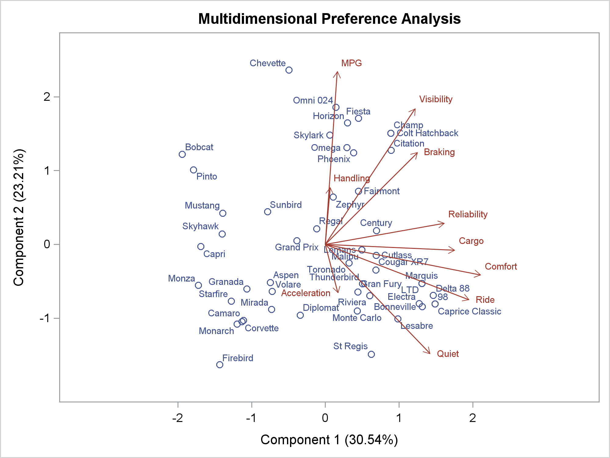
The ODS OUTPUT statement creates a data set from the data object that PROC PRINQUAL used to create the MDPREF plot. (The data object contains the coordinates of the points and vectors in the graph.)

The following step uses PROC SGPLOT and the ODS output data set from PROC PRINQUAL to re-create the MDPREF plot.

proc sgplot data=m noautolegend;
   scatter y=prin2 x=prin1 / datalabel=idlab1 datalabelattrs=graphdata1;
   vector y=vec2 x=vec1 / datalabel=label2var lineattrs=graphdata2
                          datalabelattrs=graphdata2;
   xaxis offsetmax=0.05 offsetmin=0.15;
run;

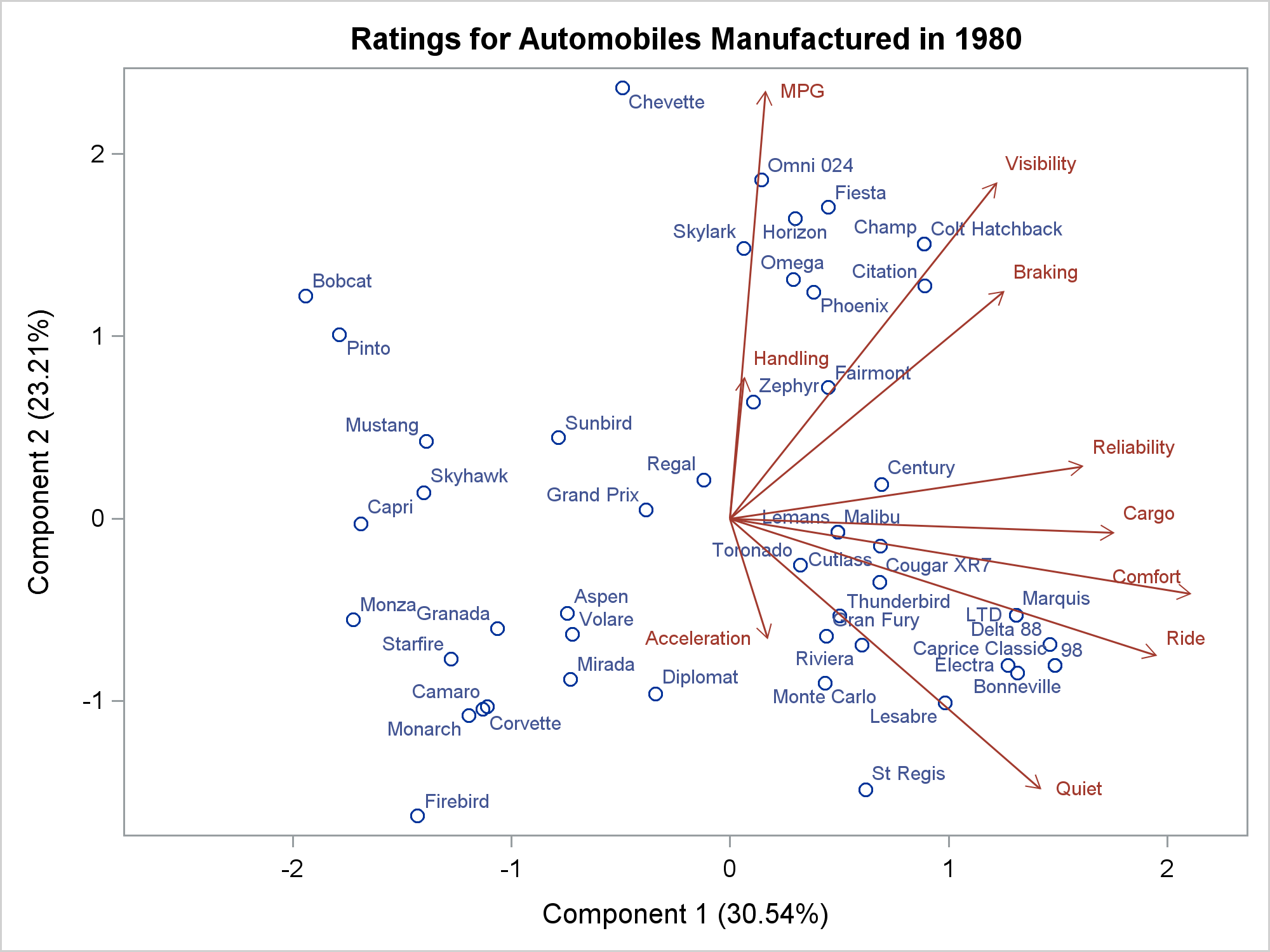
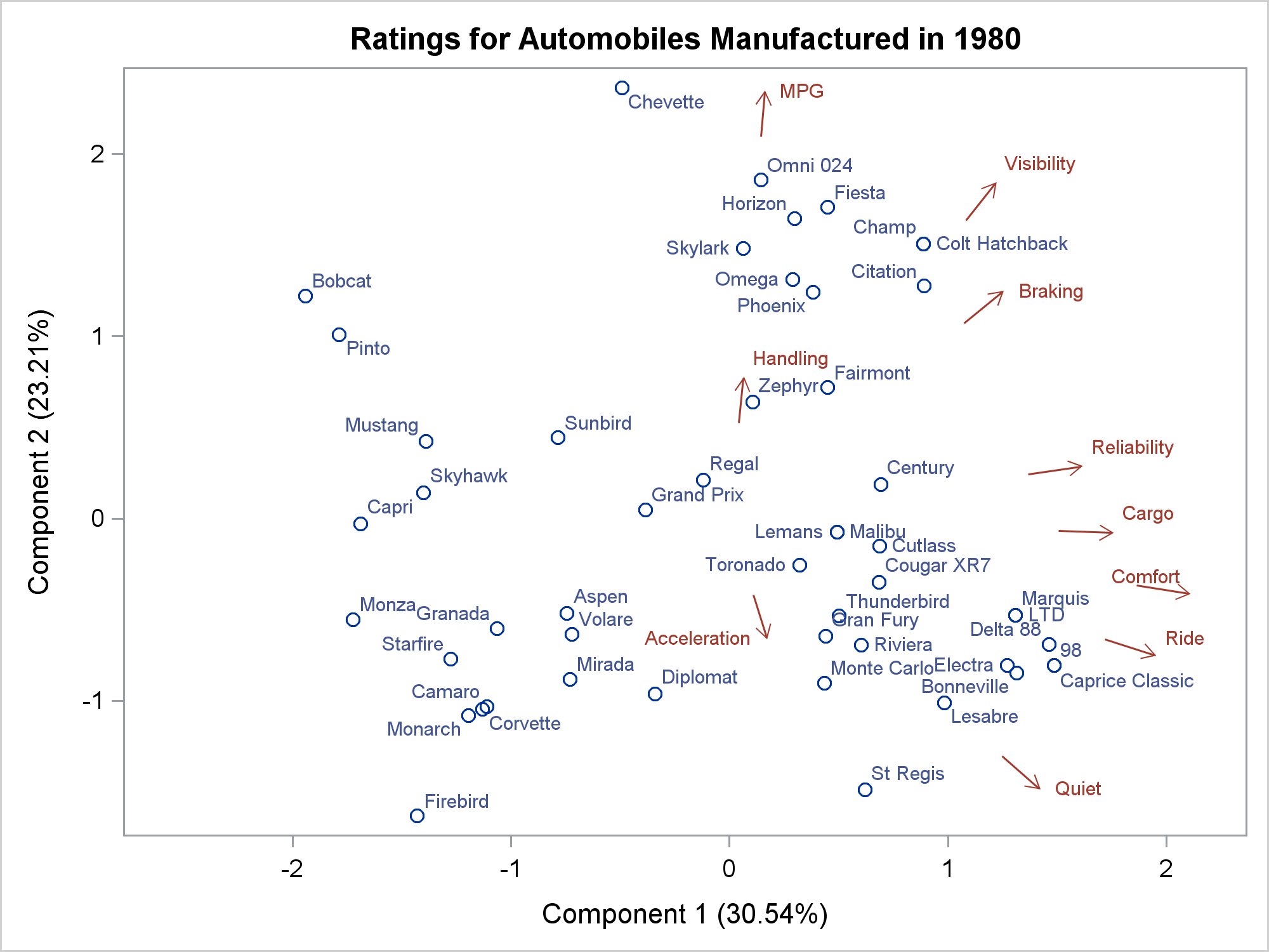
The two graphs are similar. They are not identical because the graph template that PROC PRINQUAL uses has options that I did not specify in PROC SGPLOT. In particular, PROC PRINQUAL creates a graph that has equated axes (a centimeter on the X axis represents the same data range as a centimeter on the Y axis). The following step creates new origins, one for each vector.

data m2;
   set m;
   if n(vec1, vec2) = 2 then do;
      xo = vec1 - 0.25 / sqrt(1 + (vec2 / vec1) ** 2);
      yo = (vec2 / vec1) * xo;
   end;
run;

The DATA step finds a point on the line defined by each vector that is 0.25 data units from the end of the vector (in the direction of the origin). These points are used as the origin for each vector. Each new origin is based on a slope of the line connecting (x1,y1) and (0,0), which is given by (y1 - 0) / (x1 - 0) = y1 / x1, and a new X coordinate for the origin of x1 - 0.25 sqrt{1 + (y1 / x1)**2}. Given an intercept of 0, each new Y coordinate for the origin equals the new X coordinate times the slope. This step displays the new vectors, which use the new origins (YORIGIN=YO and XORIGIN=XO).

proc sgplot data=m2 noautolegend;
   scatter y=prin2 x=prin1 / datalabel=idlab1 datalabelattrs=graphdata1;
   vector y=vec2 x=vec1 / yorigin=yo xorigin=xo
                          datalabel=label2var lineattrs=graphdata2
                          datalabelattrs=graphdata2;
   xaxis offsetmax=0.05 offsetmin=0.15;
run;

The following step creates the same vectors as the previous step and explicitly positions the center of each vector label 0.08 data units beyond the end of each vector.

data m2;
   set m;
   if n(vec1, vec2) = 2 then do;
      xo = vec1 - 0.25 / sqrt(1 + (vec2 / vec1) ** 2);
      yo = (vec2 / vec1) * xo;
      xc = vec1 + 0.08 / sqrt(1 + (vec2 / vec1) ** 2);
      yc = (vec2 / vec1) * xc;
   end;
run;
 
proc sgplot data=m2 noautolegend;
   scatter y=prin2 x=prin1 / datalabel=idlab1 datalabelattrs=graphdata1
                             markerattrs=(symbol=circlefilled size=5px);
   vector  y=vec2 x=vec1   / yorigin=yo xorigin=xo lineattrs=graphdata2;
   scatter y=yc   x=xc     / markerchar=label2var
                             markercharattrs=graphdata2;
   xaxis offsetmax=0.05 offsetmin=0.15;
run;

In this PROC SGPLOT step, the VECTOR statement does not produce any labels. Instead, a second SCATTER statement centers labels at the specified coordinates.

The following steps explicitly adjust the positions of the vector labels in the vicinity of the bottom-right quadrant.

data m2;
   set m;
   if n(vec1, vec2) = 2 then do;
      xo = vec1 - 0.25 / sqrt(1 + (vec2 / vec1) ** 2);
      yo = (vec2 / vec1) * xo;
      xc = vec1 + 0.08 / sqrt(1 + (vec2 / vec1) ** 2);
      yc = (vec2 / vec1) * xc;
      if label2var =: 'Rel' then     xc +  .18;
      if label2var =: 'Car' then     xc +  .1;
      if label2var =: 'Com' then     xc +  .15;
      if label2var =: 'Acc' then do; xc + -.32; yc +  0.10; end;
      if label2var =: 'Rid' then do; xc +  .05; yc + -0.05; end;
   end;
run;
 
proc sgplot data=m2 noautolegend;
   scatter y=prin2 x=prin1 / datalabel=idlab1 datalabelattrs=graphdata1
                             markerattrs=(symbol=circlefilled size=5px);
   vector  y=vec2 x=vec1   / yorigin=yo xorigin=xo lineattrs=graphdata2;
   scatter y=yc   x=xc     / markerchar=label2var
                             markercharattrs=graphdata2;
   xaxis offsetmax=0.05 offsetmin=0.15;
run;

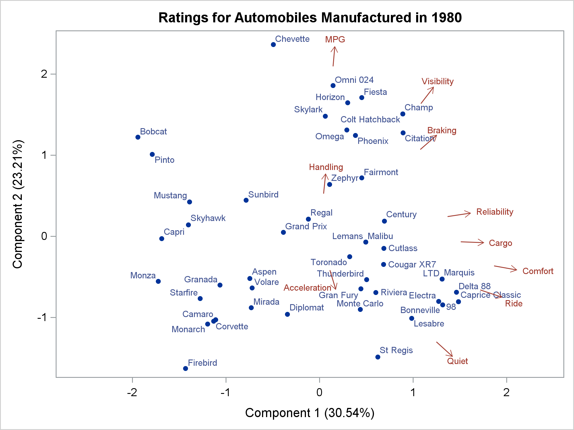
I like this final graph much more than the original graph. Changing the origin is easy. Changing the label positions is harder and ad hoc. However, if you are making a graph for a report or journal, you might want to take the extra time to explicitly move the labels to a more aesthetically pleasing location like I did here. Ad hoc label placement is covered in more detail in my free web book Advanced ODS Graphics Examples.