This is the 2nd installment of the "Getting Started" series, and the audience is the user who is new to the SG Procedures. It is quite possible that an experienced users may also find some useful nuggets here.

One of the most popular and useful graph types is the Bar Chart.  The SGPLOT procedure supports many types of bar charts, each suitable for some specific use case.  Today, we will discuss the most common type, the venerable VBAR statement.  In this article I will show you many small examples of bar charts with increasing information.

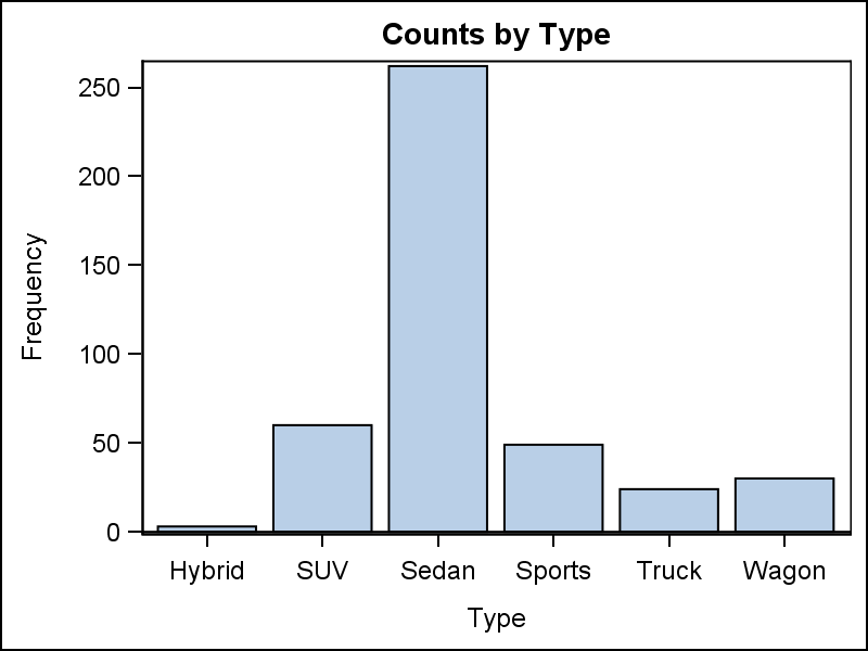Let us start with the most basic case, as shown on the right.  This graph shows the frequency or counts by category with default settings.  Click on the graph for a higher resolution image.  The SGPLOT code needed to create is very simple, as shown below.

title 'Counts by Type';
proc sgplot data=sashelp.cars;
  vbar type;
run;

The graph above is rendered to the LISTING destination with default style and default setting for the axes.

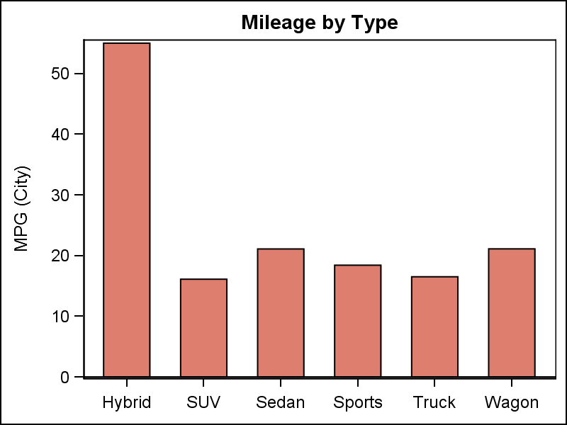The graph on the right shows the mean of city mileage by type.  The title already mentions "Mileage by Type", so there is no need to repeat that information as the label of the x-axis.  The label is suppressed by the x-axis option.

title 'Mileage by Type';
proc sgplot data=sashelp.cars;
  vbar type / response=mpg_city stat=mean
           barwidth=0.6 fillattrs=graphdata2;
  xaxis display=(nolabel);
run;

Note, we have specified RESPONSE=mpg_city, with STAT=MEAN.  This has to be set as the default STAT is SUM, and there is no point in viewing the sum of the mileage of all cars of one type.  Also, we have set BARWIDTH=0.6 and set the bar attributes to GRAPHDATA2 for a change of pace.

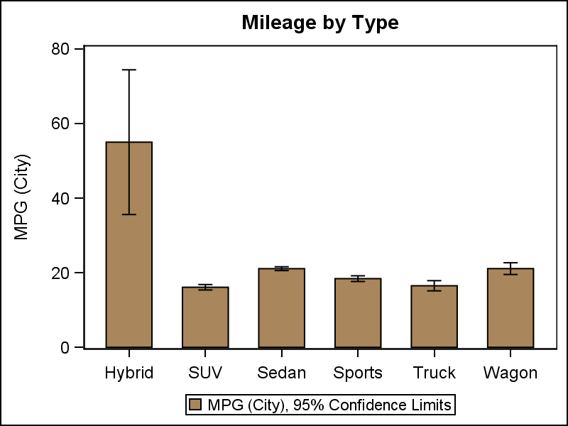Next, we create a bar chart of mean mileage by type, with display of the 95% confidence limits.  A legend is automatically created by the procedure to display the two items in the graph.  Also note, I have used GRAPHDATA4 for the bar attributes, and removed the display of the baseline to clean up the display.

title 'Mileage by Type';
proc sgplot data=sashelp.cars;
  vbar type / response=mpg_city stat=mean
            barwidth=0.6
            fillattrs=graphdata4 limits=both
            baselineattrs=(thickness=0);
  xaxis display=(nolabel);
run;

The graph on the right shows the mean mileage by type, using options to create a different look and feel.  We have also displayed the response value for each bar at the top.  A decorative skin is used to make the bars aesthetically pleasing using DATASKIN=matte.

In this graph I have suppressed the border around the data area.  The axis lines and ticks are removed and y-axis grids are added.  This results in a clean graph as shown on the right.  Click on the graph for a higher resolution image.

title 'Mileage by Type';
proc sgplot data=sashelp.cars noborder;
  format mpg_city 4.1;
  vbar type / response=mpg_city stat=mean
           datalabel dataskin=matte
           baselineattrs=(thickness=0)
           fillattrs=(color=&softgreen);
  xaxis display=(nolabel noline noticks);
  yaxis display=(noline noticks) grid;
run;

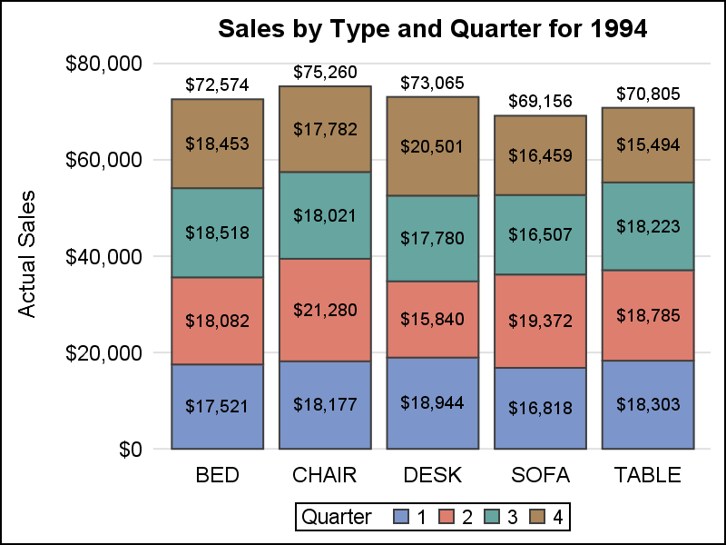Now, let us add a group classifier using the GROUP=variable option.  The SGPLOT procedure summarizes the response data by category and group.  Values for each group are stacked for each category, creating a stacked bar chart as shown on the right.

title 'Sales by Type and Quarter for 1994';
proc sgplot data=sashelp.prdsale(where=(year=1994)) noborder;
  format actual dollar8.0;
  vbar product / response=actual stat=sum
           group=quarter seglabel datalabel
          baselineattrs=(thickness=0)
          outlineattrs=(color=cx3f3f3f);
  xaxis display=(nolabel noline noticks);
  yaxis display=(noline noticks) grid;
run;

A stacked bar chart makes sense with STAT=SUM (default).  Now the bar height is the sum of all the observations for the category.  By default, SGPLOT stacks the segments for each group in a category.  Note, with SAS 9.4, the segments can be labeled with the value of each segment, and the bar itself can also be labeled with the total value for each bar.  Note, a legend showing the color used for each unique value of the group variable is shown.

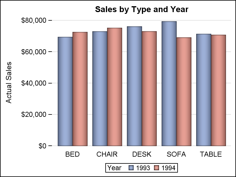Another useful graph is shown on the right.  Here, we have used GROUPDISPLAY=CLUSTER which places the groups side-by-side within each category.  A group legend is displayed by default.

title 'Sales by Type and Year';
proc sgplot data=sashelp.prdsale noborder;
  vbar product / response=actual
          group=year groupdisplay=cluster
         dataskin=pressed
         baselineattrs=(thickness=0);
  xaxis display=(nolabel noline noticks);
  yaxis display=(noline) grid;
run;

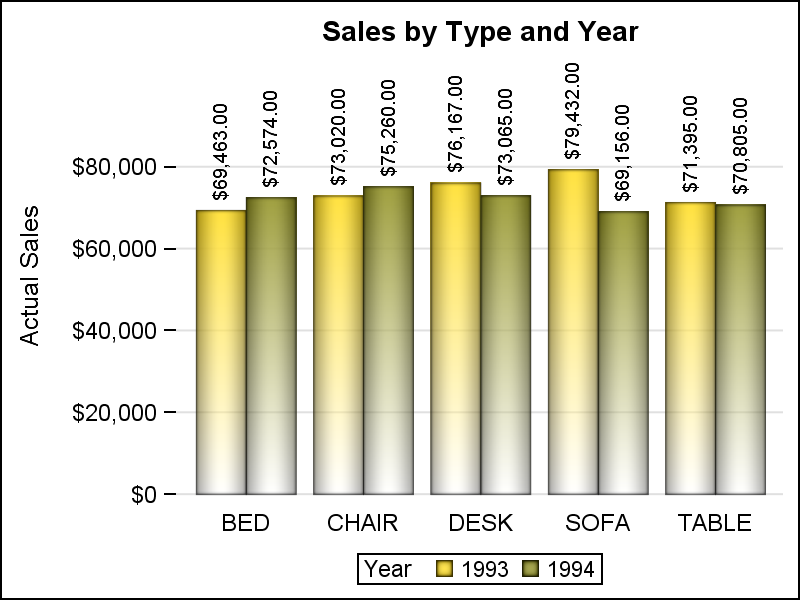Bar values can be shown for each group in a category, as shown on the right.  Note, the values are automatically rotated to a vertical orientation when the values will not fit in the space available.

Note the use of the STYLEATTRS statement to set the fill colors for the two group values to gold and olive.  This statement allows to control the attributes for the group values for fill colors, contrast colors, marker symbols and line patterns.  Also, note the use of FILLTYPE=Gradient to color the bars in an alpha gradient, from fully saturated at the top, to transparent at the bottom.

title 'Sales by Type and Year';
proc sgplot data=sashelp.prdsale noborder;
  styleattrs datacolors=(gold olive);
  vbar product / response=actual  
           group=year groupdisplay=cluster
          dataskin=pressed baselineattrs=(thickness=0)
          filltype=gradient datalabel;
  xaxis display=(nolabel noline noticks);
  yaxis display=(noline) grid;
run;

You may have noted that the VBAR statement supports only one GROUP role, which can then be displayed as STACKED or CLUSTERED.  SGPLOT does not support a bar chart that has both a CLUSTER and a STACK group like the SAS/GRAPH GCHART statement.  Creating such a graph requires some complex layout of the category axis, and a decision was made to avoid such complex axis layouts as this combination is relatively rare.

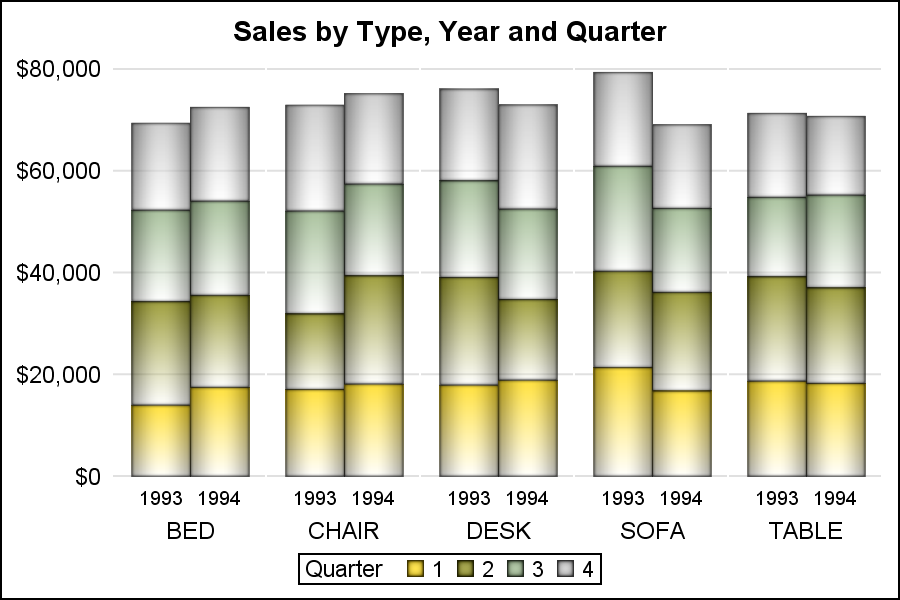But, what to do if you do need a stacked + clustered bar chart?  The solution is to use the SGPANEL procedure as shown below.  The resulting graph is shown on the right.  Here we have a bar chart of actual sales by type, year and quarter.  The year values are side-by-side and the quarter values are stacked.

The SGPANEL procedure below uses the panel variable of product.  So, each "cluster" is really a cell in the panel.  Each cell contains a stacked bar chart with category of year and group=quarter.  Normally, the cell header is at the top of each cell, with a header border.  Here, we have moved the header to the bottom of the graph, and suppressed the cell borders, thus making the graph appear like a stacked+clustered bar chart.  Note use of COLAXIS instead of XAXIS and ROWAXIS instead of YAXIS.

title 'Sales by Type, Year and Quarter';
proc sgpanel data=sashelp.prdsale;
  styleattrs datacolors=(gold olive &softgreen silver);
  panelby product / onepanel rows=1 noborder layout=columnlattice
                 noheaderborder novarname colheaderpos=bottom;
  vbar year / response=actual stat=sum group=quarter barwidth=1
           dataskin=pressed baselineattrs=(thickness=0) filltype=gradient;
  colaxis display=(nolabel noline noticks) valueattrs=(size=7);
  rowaxis display=(noline nolabel noticks) grid;
run;

For all the examples above, the data contains one or more classifier variables with one response variable.  This is what is sometimes referred to as a "Tall" structure.  But often, the data structure is "Wide", like in an Excel table, with multiple response columns by category.

In such a case, it is possible to create a clustered bar chart without transforming the data, by layering the data for each column as shown on the right.  Here, we have layered two bar VBAR statements, one for mpg_city and one for mpg_highway, both for the same category variable.  Normally, the second layers would cover the first, but we have made the 2nd layer bars narrower, so we can see both.

title 'Mileage by Type';
proc sgplot data=sashelp.cars noborder;
  styleattrs datacolors=(olive gold);
  vbar type / response=mpg_city stat=mean
           dataskin=pressed baselineattrs=(thickness=0) ;
  vbar type / response=mpg_highway stat=mean
          dataskin=pressed baselineattrs=(thickness=0)
         barwidth=0.5;
  xaxis display=(nolabel noline noticks);
  yaxis display=(noline) grid;
run;

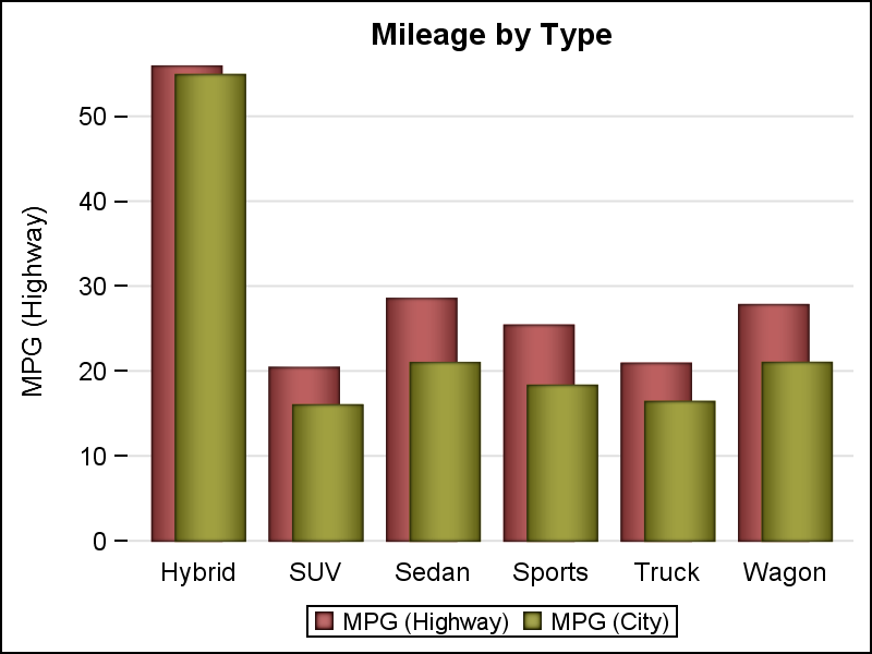Finally, the bars need not be overlayed on category centers, but can be "offset" to be side-by-side, or even a bit overlapped as shown on the right.  Here the bar widths are 0.6, and each VBAR is offset to left or right by 0.1, creating overlapping bars.

title 'Mileage by Type';
proc sgplot data=sashelp.cars noborder;
  styleattrs datacolors=(brown olive);
  vbar type / response=mpg_highway stat=mean
           dataskin=pressed barwidth=0.6 
           baselineattrs=(thickness=0)
           discreteoffset=-0.1;
  vbar type / response=mpg_city stat=mean
          dataskin=pressed barwidth=0.6 
          baselineattrs=(thickness=0)
          discreteoffset= 0.1;
  xaxis display=(nolabel noline noticks);
  yaxis display=(noline) grid;
run;

There is one restrictioin when layering multiple VBAR statements.  The category variables for all VBAR statements must be the same.  If a group is specified, it must be specified for all the VBAR statements in the same way.  If this is not the case, the program will stop with an error message in the log.  There are other ways to handle such cases that will be discussed later.

These examples give you an idea of the versatility of the SGPLOT VBAR statement.  You can create bar charts from the simplest to complex and with different aesthetic appearance.  I would encourage you to see other examples in this blog on creating bar charts with SGPLOT procedure.

Full code:  getting_started_2_vbar