In her article Creating Spaghetti Plots Just got Easy, Lelia McConnell has provided us a glimpse into some new useful features in the SAS 9.4M2 release.  The term Spaghetti plots generally refers to cases where time series plots have to be  identified by multiple group classifications.  The support for the GroupLC and GroupLP options, among others make it easy to create such graphs.

The key point to note here is that the GROUP variable is used to decide which observations in the plot should be connected.  So, the group variable should provide the finest grain classification for the series in the plot.  Normally, each individual series is rendered using one of the GraphData elements from the style, providing unique attributes to each series.

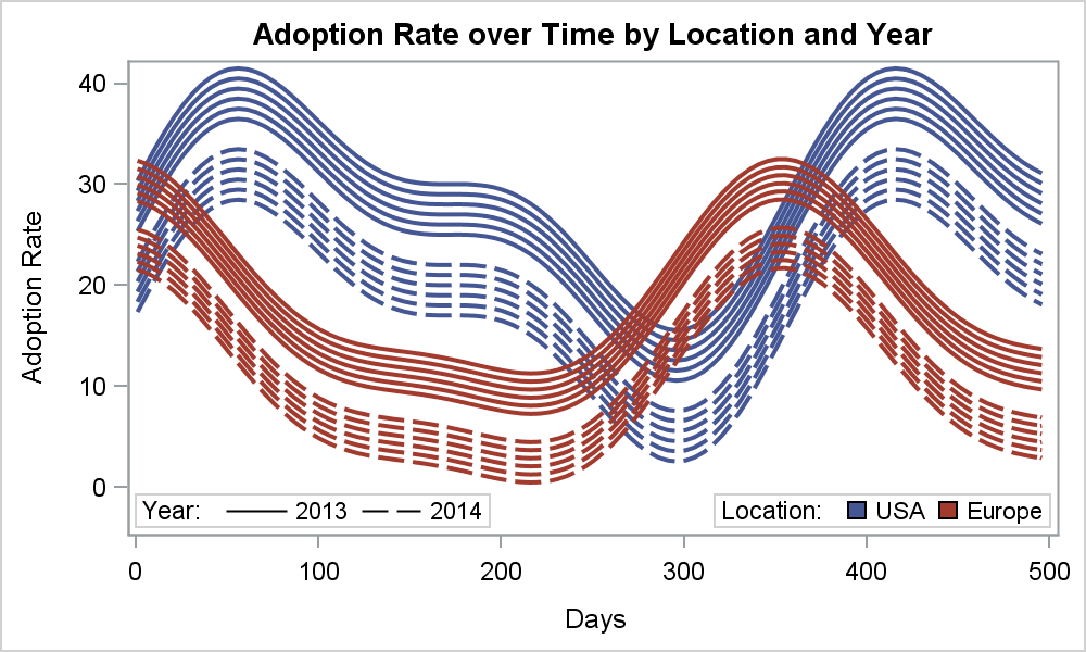However, if multiple series in the graph represent one specific value from another classifier, such as treatment or study, we can provide higher classification roles using the GroupLC  (GroupLineColor) or GroupLP (Group Line Pattern), etc., as shown in the graph on the right.  In this example, the simulated data represents the adoption rate over time for some item classified by location (color) and year (pattern) using the following code for the SERIES plot statement:

series x=x y=y / group=id lineattrs=(thickness=2 pattern=solid)
grouplc=Location grouplp=year smoothconnect;

This graph, along with other graphs using SAS 9.4M2 features are shown in the samples in the Graph Focus page on the SAS Support web site.  Now that SAS 9.4M2 is released (Aug 5), we will be adding more samples demonstrating the features at this location.

Many of you who do not yet have the SAS 9.4M2 release are asking, what does this do for me?  Well, there is good new.  While this feature has now been included in the SGPLOT procedure, it has always been available in GTL. Here is the GTL code you can use at SAS 9.4.  Note the use of the subpixel and itemsize options.

proc template;
  define statgraph MultiClassSeries;
    begingraph / subpixel=on;
      entrytitle 'Adoption Rate over Time by Location and Year';
      layout overlay / yaxisopts=(offsetmin=0.1);
        seriesplot x=x y=y / group=id name='a' lineattrs=(thickness=2) 
                             linecolorgroup=Location linepatterngroup=year;
        discretelegend 'a' / title='Location:' type=linecolor location=inside 
             valign=bottom halign=right;
        discretelegend 'a' / title='Year:' type=linepattern location=inside 
             valign=bottom halign=left itemsize=(linelength=30px);
      endlayout;
    endgraph;
  end;
run;

You can also run this with SAS 9.3, except for the subpixel and itemsize option.  Remove those, and you are good to go.

SAS 9.4 GTL code:  Spaghetti