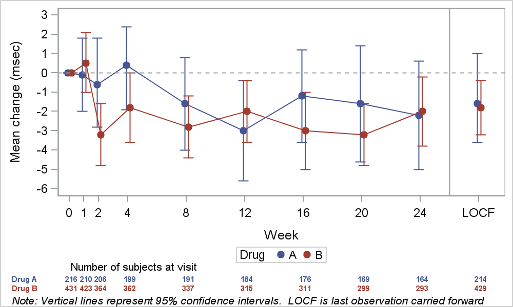
A key element of graphs used for analysis of safety data for clinical research is the inclusion of statistical data (or tables) about the study that are aligned with the x axis of the graph.  A common example of this comes from the paper "Graphical Approaches to the Analysis of Safety Data from Clinical Trials, Pharmaceut. Statistics, 2008." by Amit Ohad, et. al. shown below.  Click on graph to see full size.

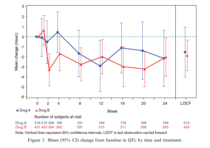
As you can see in the graph, the number of subjects at visit by treatment  is displayed at the bottom of the graph aligned with the x axis values.  Such a risk table is also very popular with Survival Plots.  Let us examine how to create such a graph, starting with the basic plot of the data itself.

QTc Mean Plot.  The basic QTC Mean plot is relatively straightforward.  Here is the simulated data that I use to create it:

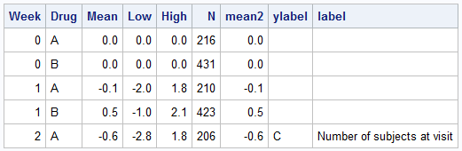
For this graph, we only need the Week, Drug, Mean, Low, High and Mean2 columns.

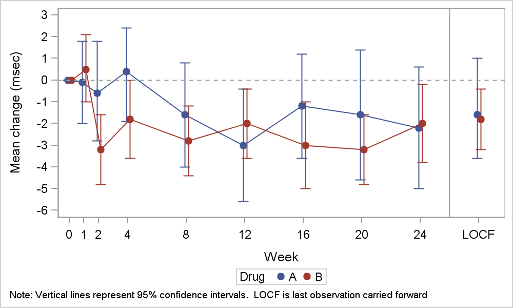
SAS 9.3 QTc Mean Graph Code:

footnote j=l h=0.8 "Note: Vertical lines represent 95% confidence intervals."
    " LOCF is last observation carried forward";
proc sgplot data=QTc_Mean_Group;
  format week qtcmean.;
  scatter x=week y=mean / yerrorupper=high yerrorlower=low group=drug
      groupdisplay=cluster clusterwidth=0.5
      markerattrs=(size=7 symbol=circlefilled);
  series x=week y=mean2 / group=drug groupdisplay=cluster clusterwidth=0.5;
  refline 26 / axis=x;
  refline 0  / axis=y lineattrs=(pattern=shortdash);
  xaxis type=linear values=(0 1 2 4 8 12 16 20 24 28) max=29 valueshint;
  yaxis label='Mean change (msec)' values=(-6 to 3 by 1);
  run;

We have used a new SAS 9.3 feature - Cluster Groups, now available with both discrete and linear X axes as follows:

1. Use a Scatter plot of mean by week with group=drug, groupdisplay=cluster and clusterwidth=0.5
2. Overlay a Series plot of mean2 by week with group=drug and same groupdisplay options.
3. Note:  Group2 is used to prevent the join with the LOCF value.
4. Set reference lines and axis values to suit.

QTc Mean with Annotated Tables.

Now, we want to add the "Number of Subjects" tables at the bottom just like in the graph from the paper.  To do that, we will use the techniques described by Dan Heath in the recent article on Annotation with SAS 9.3 SGPLOT procedure.  We will create an SGANNO data set, that includes the values to be drawn using the "TEXT" function.  Here is the annotation data set:

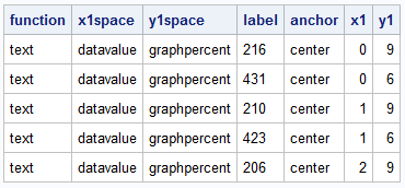
Note, the X1Space is "DataValue" because we want to align the labels with the X axis data values (0, 1, 2, 4, etc.).  The Y1Space is  "GraphPercent" because we want to place the labels at 6% and 9% from the bottom of the graph.  The annotate data set also includes the other text strings that are shown below the plot axes.  Here is the graph and the SGPLOT code:

SAS 9.3 SGPLOT Code with Annotate:

proc sgplot data=QTc_Mean_Group sganno=anno pad=(bottom=14%);
  format week qtcmean.;
  scatter x=week y=mean / yerrorupper=high yerrorlower=low group=drug
      groupdisplay=cluster clusterwidth=0.5 markerattrs=(size=7 symbol=circlefilled);
  series x=week y=mean2 / group=drug groupdisplay=cluster clusterwidth=0.5;
  refline 26 / axis=x;
  refline 0  / axis=y lineattrs=(pattern=shortdash);
  xaxis type=linear values=(0 1 2 4 8 12 16 20 24 28) max=29 valueshint;
  yaxis label='Mean change (msec)' values=(-6 to 3 by 1);
  run;

Note the use of the procedure options SGANNO=anno and PAD=(BOTTOM=14%) in the code above.  We use the pad option to create the space at the bottom, and then include the anno data set to draw the text.  The above graph is functionally equivalent to the graph in the paper.

In the graph above, the subjects table is drawn at the bottom, just above the footnotes.  My guess is the table is placed there because it is relatively easy to do with the available tools such as annotate.  The table is placed quite far from the plot, with the axis and legend in between, increasing the eye movement needed to decode the information in the graph.

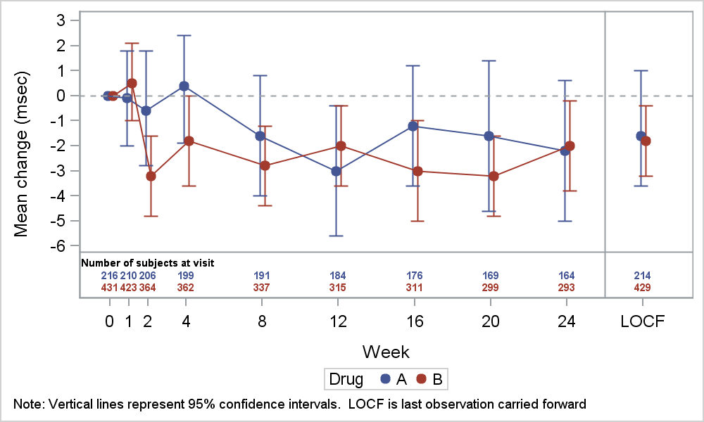
Many readers of this blog will know that you can include the "Subjects in Study" table in the graph itself using the Y / Y2 split technique discussed earlier.  Here is the  graph and the code.  Note, while this can be done using SAS 9.2 code, here we have used the SAS 9.3 feature for the cluster group overlays.

SAS 9.3 SGPLOT Code:

footnote j=l h=0.8 "Note: Vertical lines represent 95% confidence intervals."
  " LOCF is last observation carried forward";
proc sgplot data=QTc_Mean_Group;
  format week qtcmean.;
  format n 3.0;
  scatter x=week y=mean / yerrorupper=high yerrorlower=low group=drug
      groupdisplay=cluster clusterwidth=0.5 markerattrs=(size=7 symbol=circlefilled);
  series x=week y=mean2 / group=drug groupdisplay=cluster clusterwidth=0.5;
  scatter x=week y=ylabel / markerchar=label y2axis markercharattrs=(size=5 weight=bold);
  scatter x=week y=drug / group=drug markerchar=n y2axis
      markercharattrs=(size=6 weight=bold);
  refline 26 / axis=x;
  refline 0  / axis=y lineattrs=(pattern=shortdash);
  refline -6.25  / axis=y;
  xaxis type=linear values=(0 1 2 4 8 12 16 20 24 28) max=29 valueshint
      offsetmin=0.05 offsetmax=0.05;
  yaxis label='Mean change (msec)' values=(-6 to 3 by 1) offsetmin=0.18;
  y2axis display=none offsetmin=0.88 reverse;
  run;

There are some benefits of using this method to create the graph:

1. One of the principles of effective graphics is to reduce the distance between items that have to be compared in a graph.  Placing the subject numbers closer to the plot reduces eye movement required to decode the graph and results (IMHO) in a more effective graph.
2. The inset of the table in the graph itself can be done using SAS 9.2.
3. If you jitter the values by treatment, this whole graph can be done using SAS 9.2.

I have had the opportunity to discuss the placement of the subjects table inside the graph with Amit Ohad, author of the paper mentioned above.  He does not see any reasons why placing the table inside the graph is in any way detrimental to the analysis.

Full SAS 9.3 Code:  AnnoRisk_SAS93_Code