This article explains how to set up and analyze a dataset for forecasting in SAS Viya with a particular emphasis on selecting lags for dynamic models. The ability to identify the correct delayed effects of factors such as promotions and advertising expenditure is often crucial when modeling real-world demand fluctuations, and PROC TSSELECTLAG can help isolate the most important lags to improve forecast accuracy.

To start, a CAS session is first opened, and a CAS-enabled library is created to read and write data in-memory:

cas mysess;
libname mylib cas sessref=mysess;

Once the CAS session and library are established, a simulated dataset can be created to illustrate how external factors might influence sales. In practice, an existing dataset would typically be used, but here we rely on a data step to produce relevant observations:

data mylib.salesdata(keep=Week AdvertisingExpenditure PromoDiscount Sales);
     call streaminit(1234);
     Level = 500;
     Trend = 1.0;
 
     array season[52] _temporary_ (
     1.10 1.05 1.00 0.95 0.90 0.95 1.00
     1.05 1.10 1.15 1.20 1.25 1.20 1.15
     1.10 1.05 1.00 0.95 0.90 0.95 1.00
     1.05 1.10 1.15 1.20 1.25 1.20 1.15
     1.10 1.05 1.00 0.95 0.90 0.95 1.00
     1.05 1.10 1.15 1.20 1.25 1.20 1.15
     1.10 1.05 1.00 0.95 0.90 0.95 1.00
     1.05 1.10 1.15
     );
 
     do Week = 1 to 104;
          AdvertisingExpenditure = round(200 + rand("normal",0,20), 0.01);
          PromoDiscount = rand("binomial",0.2,30);
 
          SeasonFactor = season[mod(week-1,52)+1];
          PromoEffect = 1 + 0.03 * lag3(PromoDiscount);
          AdvEffect = 1 + 0.0015 * lag2(AdvertisingExpenditure);
          noise = rand("normal",0,15);
 
          ExpectedSales = Level * (Trend**(Week/52)) * SeasonFactor *
          → PromoEffect * AdvEffect;
          Sales = max(int(ExpectedSales + noise), 0);
          if Week ge 4 then output;
     end;
run;

This data step defines a baseline sales level and a simple trend, then simulates annual seasonality and delayed impacts of promotions and advertising through lag2 and lag3. Random noise is added, and the dataset ultimately includes the variables Week, AdvertisingExpenditure, PromoDiscount and Sales.

To visually examine the simulated sales data over time, you can generate a time series plot using the PROC SGPLOT procedure. The following SAS code produces a simple yet informative line chart that illustrates weekly sales across the observation period:

title "Sales History and Advertising Expenditures"; 
proc sgplot data=mylib.salesdata(where=(week<52)); 
     series x=Week y=Sales / legendlabel="Sales" ;
     scatter x=Week y=Sales / colorresponse=AdvertisingExpenditure
                              colormodel=(green  yellow  red);
     yaxis label="Sales"; 
run;
title;

The resulting plot clearly illustrates the variability of weekly sales and the influence of advertising spend:

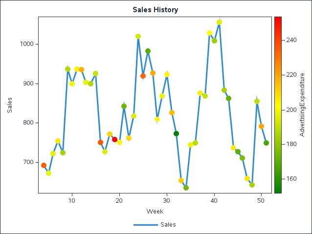
As shown in Figure 1, the marker colors, which represent advertising expenditure levels, reveal the delayed relationship between advertising and sales. Specifically, higher advertising expenditures (highlighted in red and orange tones) often precede peaks in sales by 2 periods, emphasizing the importance of including lagged advertising effects in forecasting models.

To explore the correlation of Sales with AdvertisingExpenditure and PromoDiscount across different time lags, PROC TSSELECTLAG is employed as follows:

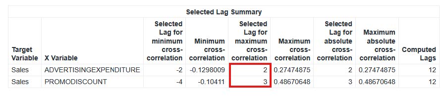
ods select results; 
ods output Results=r;
proc tsselectlag data=mylib.salesdata
                 minlag=1 
                 maxlag=12
                 correlationtype=pearson
                 out=mylib.salescorr;
     id Week; 
     yvar Sales;
     xvar AdvertisingExpenditure PromoDiscount; 
run;

By systematically testing lags from 1 through 12, this procedure calculates Pearson correlations for each specified lag. The id statement declares Week as the time dimension, while yvar and xvar set Sales as the target and AdvertisingExpenditure plus PromoDiscount as explanatory factors. The results are written to mylib.salescorr, where one can discern which lag values are most influential. The lags of AdvertisingExpenditure plus PromoDiscount with maximum cross correlation with Sales are the second and third lag, respectively.

Once meaningful lags are discovered, a forecast can be built. Potential approaches include ARIMAX or other time series models in SAS Viya, incorporating lags that reflect the actual temporal delays in your data. A valuable tool for generating forecasts is the TSMODEL procedure, which lever- ages CAS’s in-memory and parallel processing capabilities. By informing TSMODEL of the lag structure determined through PROC TSSELECTLAG, you can capture delayed effects in promotional discounts and advertising expenditure more accurately. Data preprocessing and cleansing (for instance, managing outliers or missing values) can also improve the reliability of your final forecast. Taken together, lag selection, refined demand modeling and systematic validation form a framework for dynamic demand forecasting.

Learn More