Time series data is widely used in various fields, such as finance, economics, and engineering. One of the key challenges when working with time series data is detecting level shifts. A level shift occurs when the time series’ mean and/or variance changes abruptly. These shifts can significantly impact the analysis and forecasting of the time series and must be detected and handled properly.
One popular method for detecting level shifts is using an Autoregressive Moving Average (ARMA) time series model. ARMA models are widely used in time series analysis as they combine the autoregressive (AR) and moving average (MA) components to capture both short-term and long-term dependencies in the data. By fitting an ARMA model to the time series data, it is possible to detect level shifts by estimating the model’s parameters.
The ARMA model without differencing can be represented mathematically as:
![]()
Where Xt is a stationary time series, ϵt is the white noise, c is a constant, ϕi and θi are the AR and MA parameters, respectively, and p and q are the order of the AR and MA components.
An ARMA model can capture a level shift by adding a dummy variable, a binary variable that takes on the value of 1 at the point of the level shift and 0 otherwise. This dummy variable can be multiplied by a scalar parameter, representing the level shift’s magnitude. The dummy variable is then included as an explanatory variable in the ARMA model.
The full ARMA model with the dummy variable can be represented mathematically as:
![]()
Where Xt is the time series, ϵt is the white noise, c is a constant, ϕi and θi are the AR and MA parameters, respectively, Dt is the dummy variable, δ is the magnitude of the level shift at time t, p and q are the order of the AR and MA parts. Note that we need to identify the time point t where the level shift occurs. This can be done by visual inspection, statistical estimation, and testing.
PROC TSMODEL, a SAS Visual Forecasting Procedure, and runTimeCode, an action in the Visual Forecasting Time Series Processing Action Set, can estimate the parameters of this model and identify level shifts using maximum likelihood or conditional least squares estimation. Once the model is estimated, you can use it to make predictions about future values of X, taking into account the level shift.
To estimate the period that a level shift occurs, TSMODEL utilizes a state space estimation technique that allows you to detect sudden changes/shocks to the mean value of the process. This approach involves introducing shocks into the model, which represent sudden changes in the mean value of the process. The shocks/level shifts are modeled as latent variables, and the period of the level shift is also estimated by conditional least squares or maximum likelihood estimation.
In some cases, detecting a level shift using an automated procedure like TSMODEL may involve some trial and error or the time and resources required to design and run a simulation to find the correct parameters that minimize the misclassification of false positive and false negative level shifts. This is especially true when the error variation is large relative to the size of the level shift.
One approach to improving the correct classification of level shifts in the case of high error variation is to use a windowed median filter on the original series Xt. This can be implemented using the following formula:

Yt is the filtered time series, Xt is the original time series, and k is the window size. The windowed median filter replaces each value in the original time series with the median value of the surrounding values within a given window.
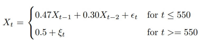
This can help to smooth out variations in the time series and make it easier to detect level shifts. We will illustrate how the median filter can improve the detection of level shifts on the following centered series. The model is simulated according to an AR(2) model with a positive level shift at 550, after which, for 180 periods, the series is normal random noise with a mean of 0.5 and a standard deviation of 0.15. The model is given by:
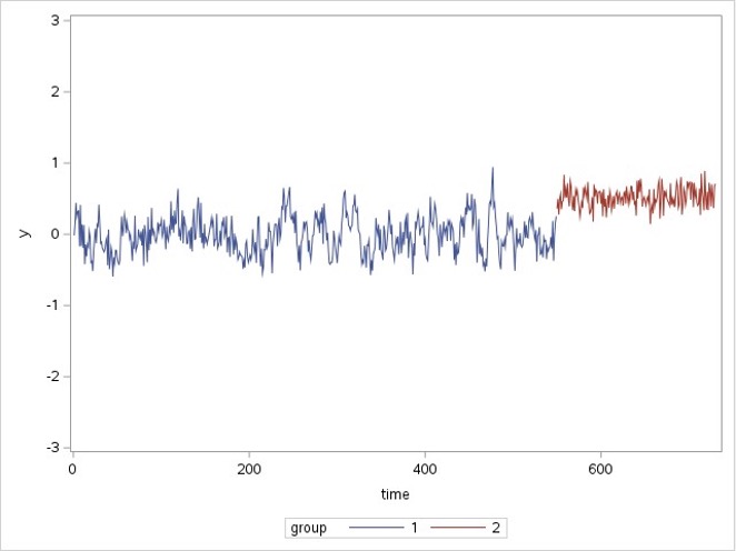
The time series plot illustrates the series and the positive level shift occurring at period 550.
We will attempt to detect the level shift using TSMODEL. Level shift detection in the time series modeling language is controlled by the setArimaxOutliers method. The code using level shift detection in this example is given in the next figure.
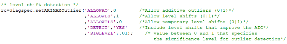
In this example, we turn on level shift detection, ALLOWTS=1, and the alpha level or type I error rate is set at SIGLEVEL=.01. The rationale for a conservative alpha level is that by visualizing the time series, it has considerable variation relative to the size of the level shift. By setting the alpha level lower, we minimize the detection of false positive level shifts due to error variation in the time series.
You can access the entire code to run the example in this article on GitHub.
After fitting the model, we can see an ARMA(1,1) model was selected, and the parameters were estimated successfully. However, the positive level shift at period 550 was not detected.

To evaluate the effect of the level shift not being detected, we will visually investigate the effect of the model, without the level shift, on the forecast 170 periods before the end of the series. The onset of the level shift occurs 180 periods before the end of the series. Let’s see how the forecast adjusts ten periods after the beginning of the level shift.
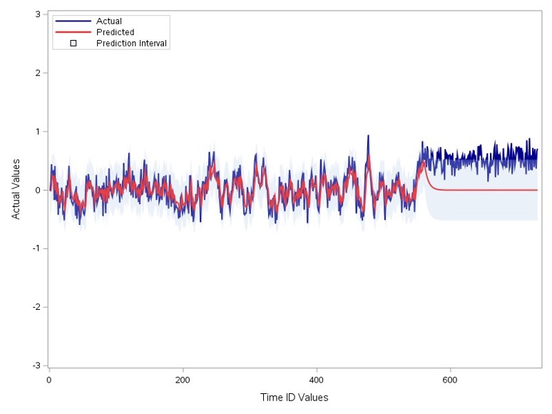
The time series plot shows that the forecast does not adjust after ten periods from the beginning of the level shift. Now we will smooth the series with the median filter using the DFMEDFILT function in SAS/IML.
We will estimate the time series model using the smoothed series as input and see if the level shift can be detected. The window size k is set to 15 for this example based on the volatility of the simulated series. We will compare the centered median with the moving average to see which adjusts faster to the level shift in the original series.
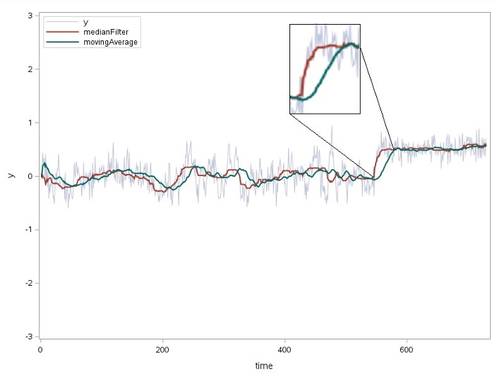
The median filtered series is the red series, and the moving average series is the green series. The viewport in the plot that zooms into the level shift at period 550 shows that the median filtered series adapts faster to the level shift. We will utilize the median filtered series as input to TSMODEL to see if the level shift can be detected.
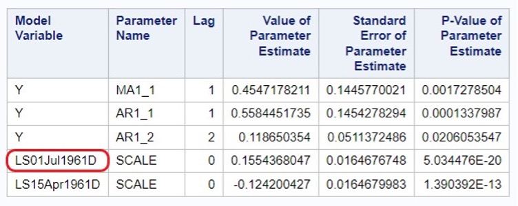
The parameter estimates from the median filtered series model indicate that an ARMA(2,1) model with two level shifts was selected. The most significant level shift is associated with the positive level in the actual series. This level shift was detected to occur four days before the actual level shift occurred. Any forecast after this period will account for the level shift, unlike the ARMA(1,1) model on the original series that did not adapt even ten periods after the onset. The median-filtered model also detected a spurious false positive level shift before the true level shift.
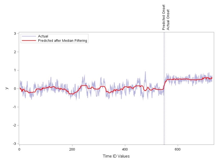
The forecast plot below illustrates that the level shift was captured, and the difference between the actual onset of the level shift and the predicted onset is relatively small.
You can find the code in this article on the public SAS® software GitHub.
References
SAS® Viya® Programming Documentation, Advanced Analytics, IML (Interactive Matrix Language), SAS/IML, SAS/IML User’s Guide, Language Reference, Statements, Functions, and Subroutines, DFMEDFILT function
https://go.documentation.sas.com/doc/en/pgmsascdc/v_034/imlug/imlug_langref_sect117.htm
Wicklin R., The Do Loop, The running median as a time series smoother The running median as a time series smoother - The DO Loop (sas.com)
Wicklin R., The Do Loop, What is a moving average? What is a moving average? - The DO Loop (sas.com)
John C. Brocklebank, David A. Dickey, Bong S. Choi, SAS for forecasting time series, Third edition, Cary, NC : SAS Institute, 2018