The running median as a time series smoother

When data contain outliers, medians estimate the center of the data better than means do. In general, robust estimates of location and sale are preferred over classical moment-based estimates when the data contain outliers or are from a heavy-tailed distribution. Thus, instead of using the mean and standard deviation of data, some analysts prefer to use robust statistics such as the median, the trimmed mean, the interquartile range, and the median absolute deviation (MAD) statistic.

A SAS statistical programmer recently wanted to use "rolling" robust statistics to analyze a time series. The most familiar rolling statistic is the moving average, which is available in PROC EXPAND in SAS/ETS software. In addition to rolling weighted means, the EXPAND procedure supports a rolling median, which is shown in the next section. However, it does not compute a robust rolling estimate of scale, such as a rolling MAD statistic. However, you can use PROC IML to compute robust estimates.

This article discusses how to compute robust rolling statistics for a time series. A subsequent article will discuss the rolling MAD statistic, which enables you to identify outliers in a time series.

An example of a rolling median

The following example shows how to compute a running median in SAS. The data (from Velleman and Hoaglin, 1981, p. 161ff) are the daily temperature of a cow (measured by counting chirps from a telemetric thermometer). Peak temperatures are associated with estrus, which is followed by ovulation, so dairy farmers want to estimate the peaks of the time series to predict the best time to impregnate the cows. One simple technique is to compute the rolling median. Although a farmer would probably use a rolling window that looks back in time (such as the median of the last seven days), this example uses a seven-day centered time window to compute the rolling median:

/* Daily temperature of a cow at 6:30 a.m. measured by counting 
   chirps from a telemetric thermometer implanted in the cow. 
   y = (chirps per 5-minute interval) - 800. 
   Peak temperatures are associated with estrus, which is followed by ovulation.
   Cows peak about every 15-20 days. Source: Velleman and Hoaglin (1981). */
data Cows;
input y @@;
Day + 1;
datalines;
60 70 54 56 70 66 53 95 70 69 56 70 70 60 60 60 50 50 48 59
50 60 70 54 46 57 57 51 51 59 42 46 40 40 54 47 67 50 60 54
55 50 55 54 47 48 54 42 43 62 49 41 45 40 49 46 54 54 60 58
52 47 53 39 55 45 47 41 48 42 45 48 52 49 53
;
 
proc expand data=Cows out=MedOut method=NONE;
   id Day;
   convert y = RunMed / transformout=(cmovmed 7);  /* Centered MOVing MEDian on a 7-day window */
run;
 
title "Overlay Running Median";
title2 "Window Length = 7";
proc sgplot data=MedOut noautolegend;
   scatter x=Day y=y;
   series x=Day y=RunMed;
   xaxis grid values=(0 to 80 by 10);
   yaxis grid label="Chirps (Body Temperature)";
run;

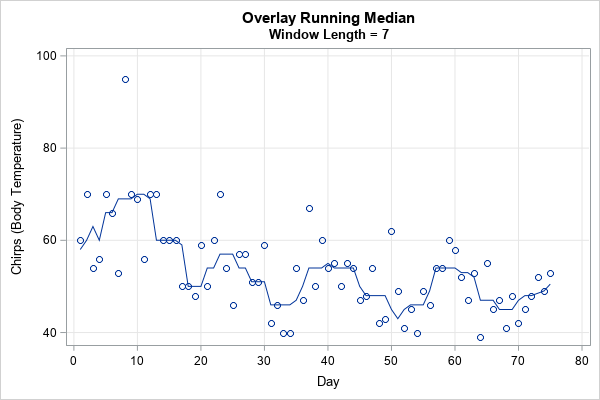
The graph overlays the rolling median on the time series of the cow's temperature. Days 10, 24, 40, and 60 are approximate peaks of the cow's temperature. Inseminating a cow after a peak is an effective strategy to impregnate a cow. The moving median smooths the cow's daily temperatures and makes the trends easier to visualize. Furthermore, a MOOO-ving median is easy to cow-culate.

Compute rolling windows in SAS/IML

I previously showed how to implement rolling statistics in the SAS/IML language. The typical technique is to

For each time point, extract the data within the time window for that time point. For example, the previous example uses a seven-day centered window.
Compute statistics for the data in each window.

If you want to compute several statistics on the same data, it can be advantageous to form a matrix that contains the data in each window. If the time series contains n observations, and each window contains L data values, then you can form the L x n matrix whose columns contain the data in the windows. You can then compute multiple statistics (means, standard deviations, medians, MADs, ....) on the columns of the matrix. For centered windows, you must decide what data to use for the first few and last few data points in the series. Two popular choices are to use missing values or to repeat the first and last points. I use the term Tukey padding to indicate that a series has been padded by repeating the first and last values.

Extract data for each window

This section shows one way to extract the data in the n windows. The following SAS/IML function pads the time series by using a user-defined value (usually a missing value) or by using Tukey padding. It then forms the (2*k+1) x n matrix whose i_th column is the window of radius k about the point y[i]:

proc iml;
/* extract the symmetric sequence about x[i], which is x[i-k-1:i+k+1] if
   1 <= i-k-1  and  i+k+1 <= nrow(x).
   Otherwise, pad the sequence. You can pad with a user-defined value 
   (such as missing or zero) or you can repeat the first or last value.
   This function loops over the number of columns and extracts each window.
   INPUT: y is the time series
          k is the radius of the window. The window length is 2*k+1 centered at y[i]
          padVal can be missing or a character value. If character,
                 use y[1] to pad on the left and y[n] to pad on the right.
*/
start extractWindows(y, k, padVal="REPEAT");
   n = nrow(y);
   M = j(2*k+1, n, .);
   /* create new series, z, by padding k values to the ends of y */
   if type(padVal)='N' then
      z = repeat(padVal, k) // y // repeat(padVal, k); /* pad with user value */
   else
      z = repeat(y[1], k) // y // repeat(y[n], k);     /* Tukey's padding */
   do i = 1 to n;
      range = i : i+2*k;   /* centered at k+i */
      M[,i] = z[range];
   end;
   return M;
finish;
 
/* create a sample time series and extract windows of length=7 (so k=3) */
t = 1:10;
y = T(20:29);                 /* the time series is 20, 21, ..., 28, 29 */
M = extractWindows(y, 3, .);  /* missing value padding */
rowlabls = {'x_{t-3}' 'x_{t-2}' 'x_{t-1}' 'x_t' 'x_{t+1}' 'x_{t+2}' 'x_{t+3}'};
/* numeric colnames are supported in SAS/IML 15.1 */
print M[c=t r=rowlabls L="Window of Length=7"];

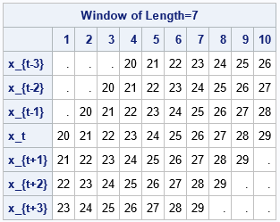
The columns of the tables show the windows for the sequence of size n=10. The windows have radius k=3 (or length 2*k+1=7), which means that the centered window at y[t]includes the points
y[t-3], y[t-2], y[t-1], y[t], y[t+1], y[t+2], and y[t+3].
Complete windows are available for t=4, 5, 6, and 7. Near the ends of the sequence (when t ≤ k or t > n-k), you must decide what data values to use in the windows. In this example, I padded the sequence with missing values. Thus, the windows about the first and last data points contain only four (not seven) data points. An alternative is to use Tukey's padding (recommended by Velleman and Hoaglin, 1981, p. 161), which pads the sequence on the left by repeating y[1] and pads the sequence on the right by repeating y[n]. Tukey's padding is the default method, so you can get Tukey's padding by calling the function as follows:

M = extractWindows(y, 3);      /* Tukey padding: Use y[1] to pad the left and y[n] to pad the right */

Apply a moving statistic to each window

Many statistics in the SAS/IML language operate on columns of a data matrix. For example, the MEAN function (which can also compute trimmed and Winsorized means) computes the mean of each column. Similarly, the MEDIAN function computes the median of each column. The following statements read the cow's temperature into a SAS/IML vector and calculates the matrix of windows of length 7, using Tukey padding. The program then computes the median and trimmed mean of each column. These rolling statistics are written to a SAS data set and plotted by using PROC SGPLOT:

use Cows; read all var {Day y}; close;
 
k = 3;
M = extractWindows(y, k);     /* Tukey padding; each column is a window of length 2*k+1 = 7 */
median = median(M);           /* compute the moving median */
mean1 = mean(M, "trim", 1);   /* compute the moving trimmed mean */
create Cows2 var{"Day", "Y", "Median", "Mean1"}; append; close;
QUIT;
 
title "Overlay Running Median and Trimmed Mean";
title2 "Window Length = 7";
proc sgplot data=Cows2;
   scatter x=Day y=y;
   series x=Day y=Median / legendlabel="Running Median(7)"
                    lineattrs=(thickness=2 color=DarkGreen);
   series x=Day y=Mean1 / legendlabel="Running Trimmed Mean(7)"
                    lineattrs=(thickness=2 color=DarkRed);
   xaxis grid;
   yaxis grid label="Chirps (Body Temperature)";
run;

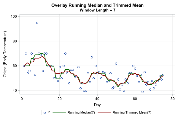
The graph overlays two rolling robust statistics on the cow's temperature for each day. The rolling median is the same as is produced by PROC EXPAND except for the first and last k observations. (PROC EXPAND uses missing-value padding; the SAS/IML example uses Tukey padding.) The rolling trimmed mean is a different robust statistic, but both methods predict the same peaks for the cow's temperature.

Summary

A rolling median is a robust statistic that can be used to smooth a time series that might have outliers. PROC EXPAND in SAS/ETS software supports the rolling median. However, you can also use SAS/IML to construct various rolling statistics.

This article shows how to use PROC IML to construct a matrix whose columns are moving windows. You can choose from two different ways to populate the windows at the beginning and end of the series. After you compute the matrix, you can apply many classical or robust statistics to the columns of the matrix. This gives you a lot of flexibility if you want to construct robust rolling statistics that are not supported by PROC EXPAND. This article shows an example of a trimmed mean. A second article discusses how to use the MAD statistic to identify outliers in a time series.

Blogs