It is well known that classical estimates of location and scale (for example, the mean and standard deviation) are influenced by outliers. In the 1960s, '70s, and '80s, researchers such as Tukey, Huber, Hampel, and Rousseeuw advocated analyzing data by using robust statistical estimates such as the median and the median absolute deviation (MAD) from the median. A common theme in this research was to use robust estimates to identify and exclude outliers. If you are not familiar with the MAD statistic, see the Appendix at the end of this article for an overview and references.

Detecting outliers: The classical approach

Suppose you have a time series that might have outliers in it. A simple method to detect outliers is to estimate the rolling center of the time series by fitting a smooth curve to the series. You can then classify an observation as an outlier if it is sufficiently far away from the curve. For example, you might classify an outlier as a point, y[t], such that |y[t]- mean[t]| > 3*std[t], where mean[t]is the moving average at t (using some window length) and std[t]is the moving standard deviation.

Unfortunately, the classical moving average and moving standard deviation are influenced by the outliers. Consequently, you might not be able to detect the outliers if you use a moving average as the smoother and use a moving standard deviation to determine "far away." The following example shows how classical estimates can fail to detect outliers. In the example, most observations are on a sine curve except for four outliers that are artificially set to 5, which is far from the sine curve. The examples use PROC EXPAND in SAS/ETS and windows of length 7 to compute a running mean and a running standard deviation:

data Test;
pi = constant('pi');
do t = 1 to 30;
   y = sin(2*pi*t/30);
   if t in (3 12 13 24) then y = 5;
   output;
end;
run;
 
proc expand data=Test out=Classical method=NONE;
   id t;
   convert y = RunMean / transformout=(cmovave 7);
   convert y = RunStd / transformout=(cmovstd 7);
run;
 
data Classical;
   set Classical;
   lower = RunMean - 3*RunStd;  /* classical intervals: mean +/- 3*std */
   upper = RunMean + 3*RunStd;
run;
 
title "Moving Average and Standard Deviation";
proc sgplot data=Classical;
   band x=t lower=lower upper=upper / name="b" legendlabel="Classical Interval";
   scatter x=t y=y / name="data";
   series x=t y=RunMean / name="c" legendlabel="Running Mean(7)";
   keylegend "b" "c";
run;

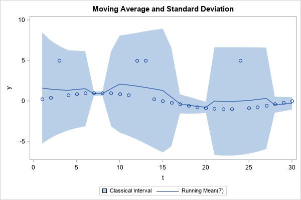
The graph overlays the data and a simple centered moving average. The shaded region shows the intervals mean[t]± 3*std[t], where mean[t]and std[t]are the moving average and moving standard deviation, respectively, at time t. You can see that the moving average is higher near the outliers. In addition, the moving standard deviation is larger near the outliers. Because of these two facts, the outliers at t={3 12 13 24} are actually INSIDE the intervals mean[t]± 3*std[t]. Thus, when you use classical (non-robust) estimates, this technique does not detect the outliers.

The Hampel identifier

If you replace the moving average and moving standard deviation with their robust counterparts (median and MAD), you obtain the Hampel identifier. Hampel suggested that observations that lie outside the moving interval median[t]± h*(1.4826*MAD[t]) be considered outliers. Most practitioners use h=3, but you can use higher values to identify more extreme outliers. The factor 1.4826 is explained in the Appendix to this article. It is chosen so that 1.4826*MAD estimates the standard deviation of normally distributed data.

A previous article shows how to use SAS/IML to compute the points in moving windows of a time series. That article defines the extractWindows function, which returns a matrix whose columns are the data in each moving window. The MAD function in SAS/IML computes the MAD of each column, so you can easily form the Hampel intervals and test which observations are outside of the intervals.

The following SAS/IML program reads the Test data and applies the Hampel identifier. The vector Outlier is a binary indicator variable; the value is 1 for observations that are outside of the robust Hampel intervals:

proc iml;
/* define or STORE/LOAD the extractWindows function. The function is defined at
   https://blogs.sas.com/content/iml/2021/05/26/running-median-smoother.html */
load module = extractWindows;
use Test; read all var {'t' 'y'}; close;
 
M = extractWindows(y, 3);   /* k=3 ==> window length=7 */
med = T( median(M) );       /* column vector of medians */
Nmad = T( mad(M, "NMAD") ); /* column vector of 1.4826*MADs */
/* Hampel identifier: Which obs are outside med +/- 3*NMAD? */
lower = med - 3*Nmad;
upper = med + 3*Nmad;
outlier = ( abs(y-med) > 3*Nmad );
 
create Robust var {'t' 'y' 'med' 'lower' 'upper' 'outlier'}; append; close;
QUIT;
 
title "Robust Moving Estimates";
title2 "Hampel Filter Using Median and MAD";
proc sgplot data=Robust;
   band x=t lower=lower upper=upper / name="b" legendlabel="Robust Interval";
   scatter x=t y=y  / name="group" group=outlier;
   series x=t y=med / name="c" legendlabel="Running Median(7)";
   keylegend "b" "c";
run;

Unlike the classical method, the robust Hampel identifier successfully flags all four unusual observations. Notice two features of the graph:

• The curve of rolling medians is closer to the underlying sine curve than the curve for rolling means.
• The robust Hampel intervals (the shaded region) are narrower than the corresponding classical intervals. The Hampel intervals are wider near the outliers (as they should be) but are small enough that the unusual observations are outside the intervals.

The Hampel identifier for real data

How well does the Hampel identifier work on real data? The previous article included data for the temperature of a cow. The following program reads the COWS data and uses the Hampel identifier to locate unusual temperatures:

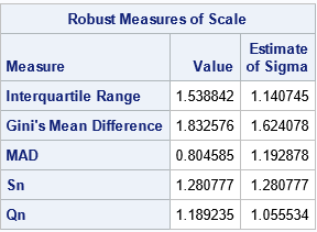
/* apply the Hampel identifier to the Cows data */
proc iml;
/* define or STORE/LOAD the extractWindows function. */
load module = extractWindows;
use Cows; read all var {Day y}; close;
 
/* Hampel identifier: Use moving median and MAD to identify outliers */
start HampelID(y, k, multiplier=3);
   M = extractWindows(y, k, "REPEAT");
   med = T( median(M) );
   Nmad = T( mad(M, "NMAD") ); 
   idx = loc( abs(y-med) > multiplier*Nmad );
   return idx;
finish;
 
idx = HampelID(y, 3);
print idx;
 
outlier = j(nrow(y), 1, 0); /* most obs are not outliers */
outlier[idx] = 1;           /* these were flagged as potential outliers */

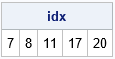
For the COWS data, the observations on days {7, 8, 11, 17, 20} are identified by the Hampel intervals as potential outliers. You can overlay the running median and Hampel intervals on the COWS data to obtain the following graph:

The graph verifies that the temperatures on days {7, 8, 11} are unusual. The temperatures on days {17, 20} are marginally outside of the Hampel intervals. As with all algorithms that identify potential outliers, you should always examine the potential outliers, especially if you plan to discard the observations or replace them with an imputed value.

The Hampel filter

Some practitioners in signal processing use the Hampel identifier to implement the Hampel filter. The filter replaces observations that are flagged as outliers with the rolling median. For example, the following SAS/IML code snippet shows how to replace outliers with the median values:

/* Hampel filter: Replace outliers with the medians */
newY = y;                 /* copy old series */
idx = loc(outlier);       /* find the indices where outlier=1 */
if ncol(idx)>0 then       /* are there any outliers? */ 
   newY[idx] = med[idx];  /* replace each outlier with the rolling median */

Summary

This article shows how to implement the Hampel identifier in SAS. The Hampel identifier uses robust moving estimates (usually the rolling median and rolling MAD) to identify outliers in a time series. If you detect an outlier, you can replace the extreme value by using the rolling median, which is a process known as the Hampel filter.

You can download the SAS program that creates all the analyses and graphs in this article.

Appendix: The MAD statistic

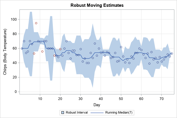
This section briefly discusses the median absolute deviation (MAD) statistic, which you can think of as a robust version of the standard deviation. For univariate data X={x1, x2, ..., xL}, the MAD is computed by computing the median (m = median(X)) and the median of the absolute deviations from the median: MAD = median(|x_i - m|). You can compute the MAD statistic (and other robust estimates of scale) by using the ROBUSTSCALE option in PROC UNIVARIATE, as follows:

proc univariate data=Test robustscale;
  var y;
  ods select robustscale;
run;

SAS also supports the MAD function in the DATA step and in PROC IML. If you are using a moving statistic, the MAD is applied to the data in each rolling window.

For a normal population, the MAD is related to σ, the population standard deviation, by the formula σ ≈ 1.4826*MAD. Therefore, if you have normally distributed data, you can use 1.4826*MAD to estimate the standard deviation. (The scale factor 1.4826 is derived in the Wikipedia article about MAD.) For example, the following SAS/IML program generates 10,000 random observations from a standard normal distribution. It computes the sample standard deviation and MAD statistics. The "NMAD" option automatically multiplies the raw MAD by the appropriate scale factor. You can see that the scaled MAD is close to the standard deviation for these simulated data:

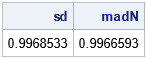
proc iml;
call randseed(4321);
x = randfun(10000, "Normal");
sd = std(x);        /* should be close to 1 */
/* for normally distributed data, 1.4826*MAD is a consistent estimator 
   for the standard deviation. */
madN = mad(x, "NMAD");  /* = 1.4826*mad, which should be close to 1 */
print sd madN;