As machine learning becomes more prevalent in financial services, one of the competing factors for adoption across organizations is the need to comply with regulatory requirements (Federal Reserve SR 11-7, Fair Housing Act, Fair Credit Reporting Act, etc.). The sticking point of regulatory compliance for newer, more complex machine learning models is that they must meet the same explainability standards of traditional models. In addition to the regulatory aspect, most executives expect predictions for models to be understandable and actionable. While much has been written about model interpretability to address these challenges, another approach is to turn a black-box model into a more interpretable model by constraining it to preserve simpler, monotonic relationships.

What are monotonic relationships?

A monotonic relationship exists when a model’s output increases or stays constant in step with an increase in your model’s inputs. Relationships can be monotonically increasing or decreasing with the distinction based on which direction the input and output travel. A common example is in credit risk where you would expect someone’s risk score to increase with the amount of debt they have relative to their income.

This makes sense to most people and has the benefit of making the relationship actionable: If you’d like a loan, reduce your debt. Imagine a non-monotonic relationship and informing some individuals to reduce their debt, while informing others to increase their debt in order to get a loan. As we can see, monotonicity can support common sense as well as fairness.

What are monotonic constraints?

Monotonic constraints are restrictions that force models to preserver monotonic relationships between a model’s inputs and its output. In the prior example, it’s a way of telling the model that the final result must show that any increase in a person’s debt-to-income ratio results in a non-decreasing change in the risk prediction.

SAS released its implementation of monotonic constraints for its Gradient Boosting procedure in Visual Data Mining and Machine Learning version 8.5. When growing a tree in SAS gradient boosting, the algorithm is constrained on each local split to enforce the monotonic relationship when this option is set. The optional setting refers to a restriction on the relationship of the input variable with the prediction function for the target event level. Therefore, if you want a decreasing relationship between a model input and output, you add a "monotonic=decreasing" option to your input statement.

How to validate monotonic relationships?

As is often the case with machine learning models, it can be hard to determine the relationship of individual variables and a prediction function from the model itself. One of the easiest ways to validate these relationships is with partial dependence (PD) plots and individual conditional expectation (ICE) plots. For more background on these plots, I highly recommend reading the detailed blog post on model interpretability. Since ICE plots occur at the observation level compared to the model average in PD plots, they could be considered more effective in validating a monotonic relationship. However, I chose to display the PD plots in this blog post for simplicity.

Monotonic constraints in action

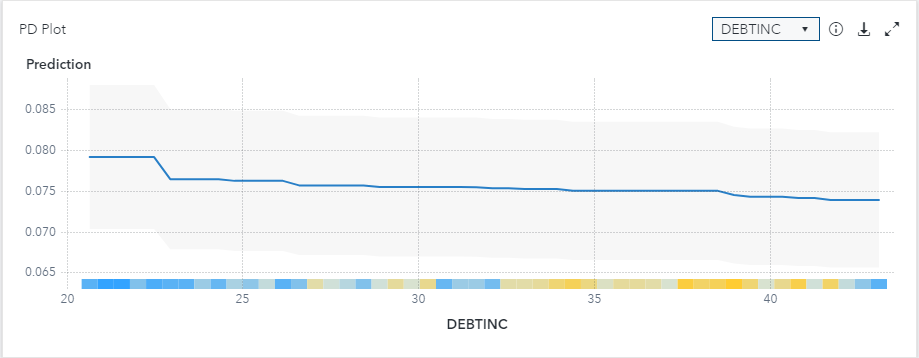
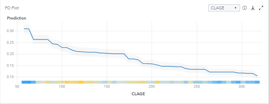
For this walk-through, I will use the ever-popular HMEQ data set from SAS which is based on HELOC loan data in a Model Studio project. I will focus on two variables that often have monotonic relationships with the probability of default: Debt-to-Income Ratio (DEBTINC – increasing relationship) and age of oldest trade line in months (CLAGE – decreasing relationship). First, we will run a standard gradient boosting model with all the default settings. We will add the Model Interpretability options to produce PD plots to depict the relationship between the input variables and the average prediction of the model. Of note for this particular data set is that the target variable "BAD" is coded as 0 and 1 with our desired predicted event level being 1, representing a bad loan. Since SAS gradient boosting defaults its event level as the first value for nominal targets (0 in our case), we will need to reverse the relationships to match our desired state.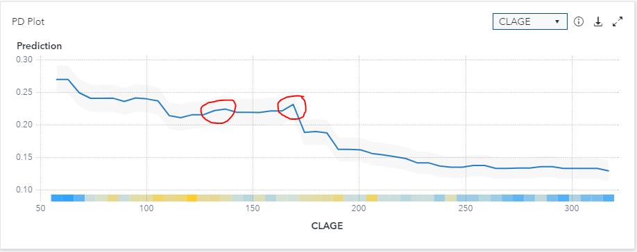

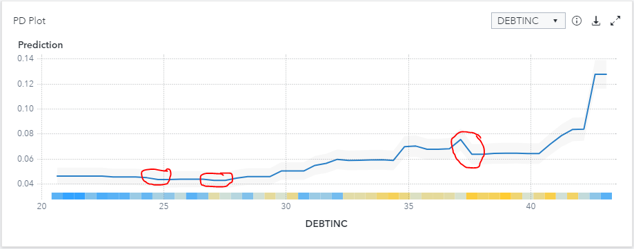
The PD plots above show that there are clear increasing and decreasing relationships with the two variables and the predicted probability of loan default. However, we would not categorize this as monotonic as there are several points in the plot that conflict with the overall direction as highlighted with the red outline. Now, we will add the monotonic constraints to see how this impacts the models.

We will first run the models with a monotonic decreasing constraint. While this option is not available in Model Studio today, we can always use a SAS code node to run the gradient boosting model with the desired option. The code below can be dropped into a SAS Code node and be run in any Model Studio pipeline as it uses the standard macros created by the software.

/* SAS code */
/* Run Gradient Boosting using gradboost procedure */
 
proc gradboost data=&dm_data
    earlystop(tolerance=0 stagnation=5 minimum=NO metric=LOGLOSS)
     binmethod=QUANTILE
     maxbranch=2
     assignmissing=USEINSEARCH minuseinsearch=1
     ntrees=100 learningrate=0.1 samplingrate=0.5 lasso=0 ridge=1 maxdepth=4 numBin=50 minleafsize=5
     seed=12345;
 
  %if &dm_num_interval_input %then %do;
    input %dm_interval_input / level=interval monotonic=decreasing;
  %end;
 
  %if &dm_num_class_input %then %do;
    input %dm_class_input/ level=nominal;
  %end;
 
  %if "&dm_dec_level" = "INTERVAL" %then %do;
    target %dm_dec_target / level=interval ;
  %end;
  %else %do;
    target %dm_dec_target / level=nominal;
  %end;
 
  &dm_partition_statement;
  ods output
    VariableImportance = &dm_lib..VarImp
    Fitstatistics      = &dm_data_outfit
  ;
  savestate rstore=&dm_data_rstore;
run;
 
/* Add reports to node results */
%dmcas_report(dataset=VarImp, reportType=Table, description=%nrbquote(Variable Importance));
%dmcas_report(dataset=VarImp, reportType=BarChart, category=Variable, response=RelativeImportance, 
              description=%nrbquote(Relative Importance Plot));

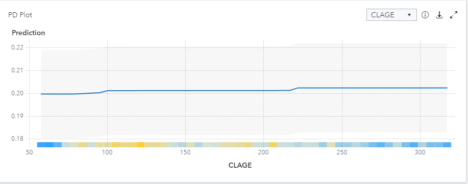
This code will develop a gradient boosting model and force a monotonic decreasing constraint on all interval variables. The PD plot below now only shows the relationship between input variables and the predicted target as increasing or constant throughout the model. However, since I've applied that relationship to all interval variables, there is a less intuitive relationship with CLAGE.

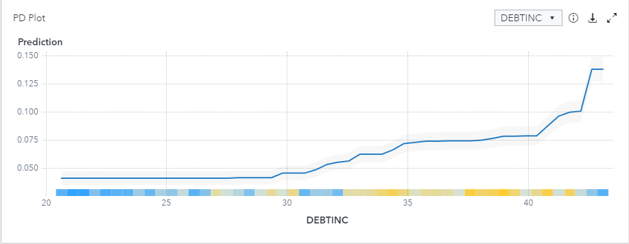
For demonstrative purposes, let’s see what happens when we tweak the code above and change the monotonic constraint from decreasing to increasing. Upon inspection of the resulting PD plots, the CLAGE plot is constrained optimally to show our desired relationship, but the DEBTINC plot is showing an undesirable relationship.

Like most real-world problems, we are seeing a mix of input variables in our dataset with varying desired relationships with our target variable. Luckily for us, SAS allows you to use multiple input statements to reflect the desired relationships in your data. The code below will enforce the monotonically increasing relationship with DEBTINC, the monotonically decreasing relationship with CLAGE, and not force any constraints on the remaining variables in the model.

/* SAS code */
/* Run Gradient Boosting using gradboost procedure */
 
proc gradboost data=&dm_data
    earlystop(tolerance=0 stagnation=5 minimum=NO metric=LOGLOSS)
     binmethod=QUANTILE
     maxbranch=2
     assignmissing=USEINSEARCH minuseinsearch=1
     ntrees=100 learningrate=0.1 samplingrate=0.5 lasso=0 ridge=1 maxdepth=4 numBin=50 minleafsize=5
     seed=12345;
 
  	input Mortdue value clno yoj / level=interval;
    input clage / level=interval monotonic=increasing;
	input debtinc / level=interval monotonic=decreasing;
 
  %if &dm_num_class_input %then %do;
    input %dm_class_input/ level=nominal;
  %end;
 
  %if "&dm_dec_level" = "INTERVAL" %then %do;
    target %dm_dec_target / level=interval ;
  %end;
  %else %do;
    target %dm_dec_target / level=nominal;
  %end;
 
  &dm_partition_statement;
  ods output
    VariableImportance = &dm_lib..VarImp
    Fitstatistics      = &dm_data_outfit
  ;
  savestate rstore=&dm_data_rstore;
run;
 
/* Add reports to node results */
%dmcas_report(dataset=VarImp, reportType=Table, description=%nrbquote(Variable Importance));
%dmcas_report(dataset=VarImp, reportType=BarChart, category=Variable, response=RelativeImportance, 
              description=%nrbquote(Relative Importance Plot));

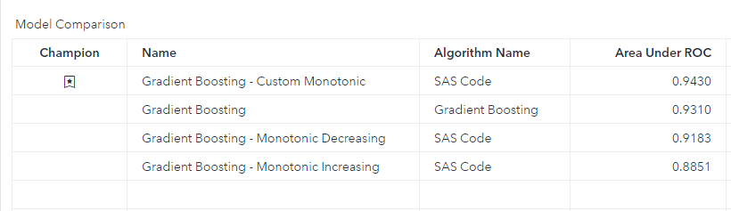
What was the result? Just as Goldilocks would say about baby bear’s bed, this model appears just right. In fact, if we examine the Model Comparison, our custom monotonic model has the highest AUC. This can often be attributed to models without certain constraints overfitting on data. The monotonic constraints in our custom model actually helped it generalize better in this instance and is not uncommon to see in real-world applications. However, oftentimes organizations are willing to sacrifice model accuracy for the benefit of a model that makes business sense and is easier to gain regulatory approval.

Conclusion

For those working in regulated industries such as financial services, I highly recommend giving gradient boosting models with monotonic constraints a shot to see if you can develop a more accurate model while adhering to regulatory guidelines.

I would like to thank Guixian Lin, Katherine Taylor, and Andrew Christian for the feedback and guidance on this post.