Getting started with deep learning using the SAS Language

Deep learning is an area of machine learning that has become ubiquitous with artificial intelligence. The complex, brain-like structure of deep learning models is used to find intricate patterns in large volumes of data. These models have heavily improved the performance of general supervised models, time series, speech recognition, object detection and classification, and sentiment analysis.

SAS has a rich set of established and unique capabilities with regard to deep learning. These capabilities can be accessed through many programming languages including Python, R, Java, Lua, and SAS, as well as through REST APIs. In this and subsequent blog posts, I’ll focus on how to use the SAS language to build deep learning models, with specific examples using different types of modeling that SAS supports.

In the examples, I use the SAS Cloud Analytic Services Language (CASL), which is called using the CAS procedure. CASL might look intimidating, but the language is actually easy to learn and use.

Before we get started, I’ll explain the three categories of deep learning models in SAS:

1) Deep feed-forward neural networks (DNN)
2) Convolutional neural networks (CNN)
3) Recurrent neural networks (RNN)

Each category has unique capabilities. In the first example below, I create a basic deep feed-forward neural network. The DNN model type is the most basic deep learning model category. The CNN and RNN variants of SAS deep learning models have characteristics that are unique for a specialized task and include capabilities far beyond the DNN type.

For instance, the CNN type consumes images as inputs. Additionally, you can use the CNN model for traditional tabular data because the CNN includes a richer subset of layers that can improve the analysis of tabular data such as batch normalization, multitask learning, reshape and so forth. A detailed description of each model type will be presented in later blogs in this series.

Here are two examples that illustrate the use DNN modeling:

Example 1: Create a basic deep feed-forward neural network model

In this example, I demonstrate how you can manually build a deep learning model architecture from scratch. I start a Cloud Analytic Services (CAS) session, assign the libref mycaslib, I load the SASHELP.BASEBALL data set as an in-memory table, and then partition the data in preparation for modeling.

proc cas;
libname mycaslib cas;
 
data mycaslib.baseball;
	set sashelp.baseball;
run;
 
proc partition data=mycaslib.baseball samppct=75    
        samppct2=25 seed=12345 partind;
     output out=mycaslib.baseball_part;
run;

Next, I use PROC CAS to specify my CAS actions. I load the Deep Learning action set called deepLearn. I’ll use multiple actions from this action set in the upcoming steps. First, I create an empty deep feed-forward neural network. You then add individual layers to the model to slowly define the network architecture. Each time you add a layer, you identify the name of the model to add the layer to, in addition to specifying the name and type of the layer. You can also specify the hyperparameters specific to the layer type, such as the activation function and the number of hidden units.

proc cas;
/* Load action set*/
loadactionset 'deeplearn';
/***************************/
/* Build a model shell		 */
/***************************/
deepLearn.BuildModel / modeltable={name='DLNN', replace=1} type = 'DNN';
/****************************/
/* Add an input layer	    */
/****************************/
deepLearn.AddLayer / model='DLNN' name='data' layer={type='input' STD='STD' dropout=.05}; 
/*********************************/
/* Add several Fully-Connected Hidden layers 	*/
/*********************************/
deepLearn.AddLayer / model='DLNN' name='HLayer1' layer={type='FULLCONNECT' n=30 act='ELU' init='xavier' dropout=.05} srcLayers={'data'};
deepLearn.AddLayer / model='DLNN' name='HLayer2' layer={type='FULLCONNECT' n=20 act='RELU' init='MSRA' dropout=.05} srcLayers={'HLayer1'};  
deepLearn.AddLayer / model='DLNN' name='HLayer3' layer={type='FULLCONNECT' n=10 act='RELU' init='MSRA' dropout=.05} srcLayers={'HLayer2'};
/***********************/
/* Add an output layer */
/***********************/
deepLearn.AddLayer / model='DLNN' name='outlayer' layer={type='output'} srcLayers={"HLayer3"};
 
quit;

Example 2: DNN with batch normalization

In this example, I create a deep feed-forward neural network that includes batch normalization layers. Check out this video for a better understanding of batch normalization, a technique that enables you to train your neural network more easily.

To incorporate batch normalization layers, I need to specify the type of model as CNN in the buildModel action.

proc cas;
deepLearn.BuildModel / modeltable={name='BatchDLNN', replace=1} type = 'CNN';
/****************************/
/* Add an input layer	    */
/****************************/
deepLearn.AddLayer / model='BatchDLNN' name='data' layer={type='input' STD='STD'}; 
/*********************************/
/* Add several Hidden layers 	*/
/*********************************/
/* 			FIRST HIDDEN LAYER 			*/
deepLearn.AddLayer / model='BatchDLNN' name='HLayer1' layer={type='FULLCONNECT' n=30 act='ELU' init='xavier'} srcLayers={'data'};
/* 			SECOND HIDDEN LAYER 		*/
deepLearn.AddLayer / model='BatchDLNN' name='HLayer2' layer={type='FULLCONNECT' n=20 act='identity' init='xavier' includeBias=False } srcLayers={'HLayer1'};
deepLearn.AddLayer / model='BatchDLNN' name='BatchLayer2' layer={type='BATCHNORM' act='TANH'} srcLayers={'HLayer2'};
/* 			THIRD HIDDEN LAYER 			*/
deepLearn.AddLayer / model='BatchDLNN' name='HLayer3' layer={type='FULLCONNECT' n=10 act='identity' init='xavier' includeBias=False } srcLayers={'BatchLayer2'};  
deepLearn.AddLayer / model='BatchDLNN' name='BatchLayer3' layer={type='BATCHNORM' act='TANH'} srcLayers={'HLayer3'};
/***********************/
/* Add an output layer */
/***********************/
deepLearn.AddLayer / model='BatchDLNN' name='outlayer' layer={type='output'} srcLayers={"BatchLayer3"};
run;
quit;

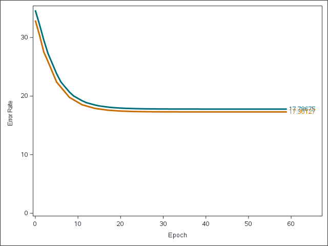
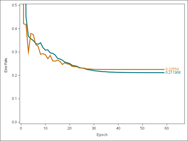
With the data uploaded and the model defined, you can begin to train the model. This next program trains the model by using the dlTrain action and creates a plot of the model fit error across iterations, with labels for the best error performance values for each partition.

ods output OptIterHistory=ObjectModeliter;
proc cas;
	dlTrain / table={name='baseball_part', where='_PartInd_=1'} model='BatchDLNN' 
        modelWeights={name='ConVTrainedWeights_d', replace=1}
        bestweights={name='ConVbestweights', replace=1}
        inputs={'CrAtBat', 'nBB', 'CrHits', 'CrRuns', 'nAtBat', 'Position','CrRbi'}
	nominals={'Position'} 
        target='logSalary'
         ValidTable={name='baseball_part', where='_PartInd_=2'} 
        optimizer={minibatchsize=5,         			algorithm={method='ADAM', beta1=0.9, beta2=0.999, learningrate=0.001, 
				lrpolicy='Step', gamma=0.5, stepsize=3}, regl1=0.00001, regl2=0.00001,
           			maxepochs=60} 
        seed=12345
;
quit;
 
 
/****************************/
/*  Store minimum training  */
/*  and validation error in */
/*  macro variables. 	    */
/****************************/
 
proc sql noprint;
	select min(FitError)
	into :Train separated by ' '
	from ObjectModeliter;
quit;
 
proc sql noprint; 
	select min(ValidError)
 	into :Valid separated by ' ' 
	from ObjectModeliter; 
quit; 
 
/* Plot Performance */
proc sgplot data=ObjectModeliter;
yaxis label='Error Rate' MAX=35 min=0;
	series x=Epoch y=FitError / CURVELABEL="&Train" CURVELABELPOS=END;
   	series x=Epoch y=ValidError / CURVELABEL="&Valid" CURVELABELPOS=END; 
 run;

How to improve deep learning performance

The model performance seems reasonable because the performance improves for a period of time and the two performance curves track well together. However, tuning the hyperparameters might improve model performance. SAS offers easy-to-use tuning algorithms to improve the deep learning model. You can surface the Hyperband approach using the dlTuneaction. DlTune is very similar to dlTrain with regards to its coding options, except you can specify upper and lower bounds for the hyperparameter search. (NOTE: SAS has improved on the original Hyperband method with regards to sampling the hyperparameter space).

proc cas;
	dlTune / table={name='baseball_part', where='_PartInd_=1'} model='BatchDLNN' 
        modelWeights={name='ConVTrainedWeights_d', replace=1}
        bestweights={name='ConVbestweights', replace=1}
        inputs={'CrAtBat', 'nBB', 'CrHits', 'CrRuns', 'nAtBat', 'Position','CrRbi'}
	nominals={'Position'} 
        target='logSalary'
         ValidTable={name='baseball_part', where='_PartInd_=2'} 
optimizer = {miniBatchSize=5, numTrials=45, tuneIter=2, tuneRetention=0.8, algorithm={method='ADAM', lrpolicy='step', 
gamma={lowerBound=0.3 upperBound=0.7},   
beta1=0.9, beta2=0.99, 
learningRate={lowerBound=0.0001 upperBound=0.01},
clipGradMax=100 clipGradMin=-100} 
regl1={lowerBound=0.0001 upperBound=0.05}
regl2={lowerBound=0.0001 upperBound=0.05}
maxepochs=10}  seed = 1234
;
quit;

DlTune’s results provide a table that contains each hyperparameter value along with the model’s performance for each respective hyperparameter combination.

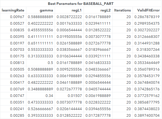
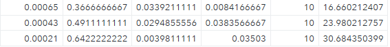
Note the large difference between the best (0.287) and worst (30.68) combinations with regards to the validation set error.

Now insert the best performing combination of hyperparameter values discovered by dlTune into the dlTrain code to retrain the model.

ods output OptIterHistory=ObjectModeliter;
proc cas;
	dlTrain / table={name='baseball_part', where='_PartInd_=1'} model='BatchDLNN' 
        modelWeights={name='ConVTrainedWeights_d', replace=1}
        bestweights={name='ConVbestweights', replace=1}
        inputs={'CrAtBat', 'nBB', 'CrHits', 'CrRuns', 'nAtBat', 'Position','CrRbi'}
	nominals={'Position'} 
        target='logSalary'
         ValidTable={name='baseball_part', where='_PartInd_=2'} 
        optimizer={minibatchsize=5, 
        			algorithm={method='ADAM', beta1=0.9, beta2=0.999, learningrate=0.00967, 
				lrpolicy='Step', gamma=0.5888888889, stepsize=3}, regl1=0.0028722222, regl2=0.0161788889,
           			maxepochs=60} 
        seed=12345
;
quit;
 
 
/****************************/
/*  Store minimum training  */
/*  and validation error in */
/*  macro variables. 	    */
/****************************/
 
proc sql noprint;
	select min(FitError)
	into :Train separated by ' '
	from ObjectModeliter;
quit;
 
proc sql noprint; 
	select min(ValidError)
 	into :Valid separated by ' ' 
	from ObjectModeliter; 
quit; 
 
/* Plot Performance */
proc sgplot data=ObjectModeliter;
yaxis label='Error Rate' MAX=35 min=0;
	series x=Epoch y=FitError / CURVELABEL="&Train" CURVELABELPOS=END;
   	series x=Epoch y=ValidError / CURVELABEL="&Valid" CURVELABELPOS=END; 
 run;

The results of the tuned deep learning model appear to be much better when compared to the original model.

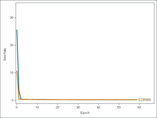
Rescaling the y-axis provides a clearer understanding of the model’s performance.

In summary, it’s easy to build and tune a deep learning model by using the SAS language. However, building a great model is not always easy, especially if you’re training a model with millions of parameters on a large amount of data. Check out this following Practitioner’s Guide video to learn a few additional tips that can help you build a good deep learning model.