This project and corresponding article were co-developed by Neela Vengateshwaran and Robert Blanchard. A follow-up article, Deployment of a Multi-stage Computer Vision model with SAS Event Stream Processing, was written by Dragos Cole.
Overview
SAS offers great flexibility using a “Bring Your Own Language” (BYOL) strategy that lets users code in the language of their choice. Brian Gaines offers an excellent introduction to building computer vision models using the SAS language for an image classification task in a community article: How to Develop SAS Code to Train a Deep Learning Model for Image Classification - SAS Support Communities. Susan Kahler details examples of leveraging SAS Deep Learning from Python using SAS DLPy in her video blog: Videos: Building computer vision models with Python and SAS Deep Learning - The SAS Data Science Blog.
This article will build upon the knowledge introduced by Brian and Susan to create a Multi-stage Computer Vision model to detect objects on high-resolution imagery taken from an aerial view. The project goal is to locate a dog, Dr. Taco, and determine if he is wearing a scarf or not and if wearing a scarf, then also determine the color of the scarf he’s wearing. We consider this to be Dr. Taco’s current “state,” and that state can change at any moment. This use case can be applied in various scenarios. For a utility company, the detection may be whether an insulator is damaged and identifying the type of damage the insulator has incurred. Drone product delivery, weather forecasting, and satellite imagery interpolation are other example use cases. The solution proposed in this article is detailed using both SAS language and Python language (through custom Python packages developed by SAS). This way, users can continue using their preferred language to leverage SAS Deep Learning capabilities.
Data Description and Challenges
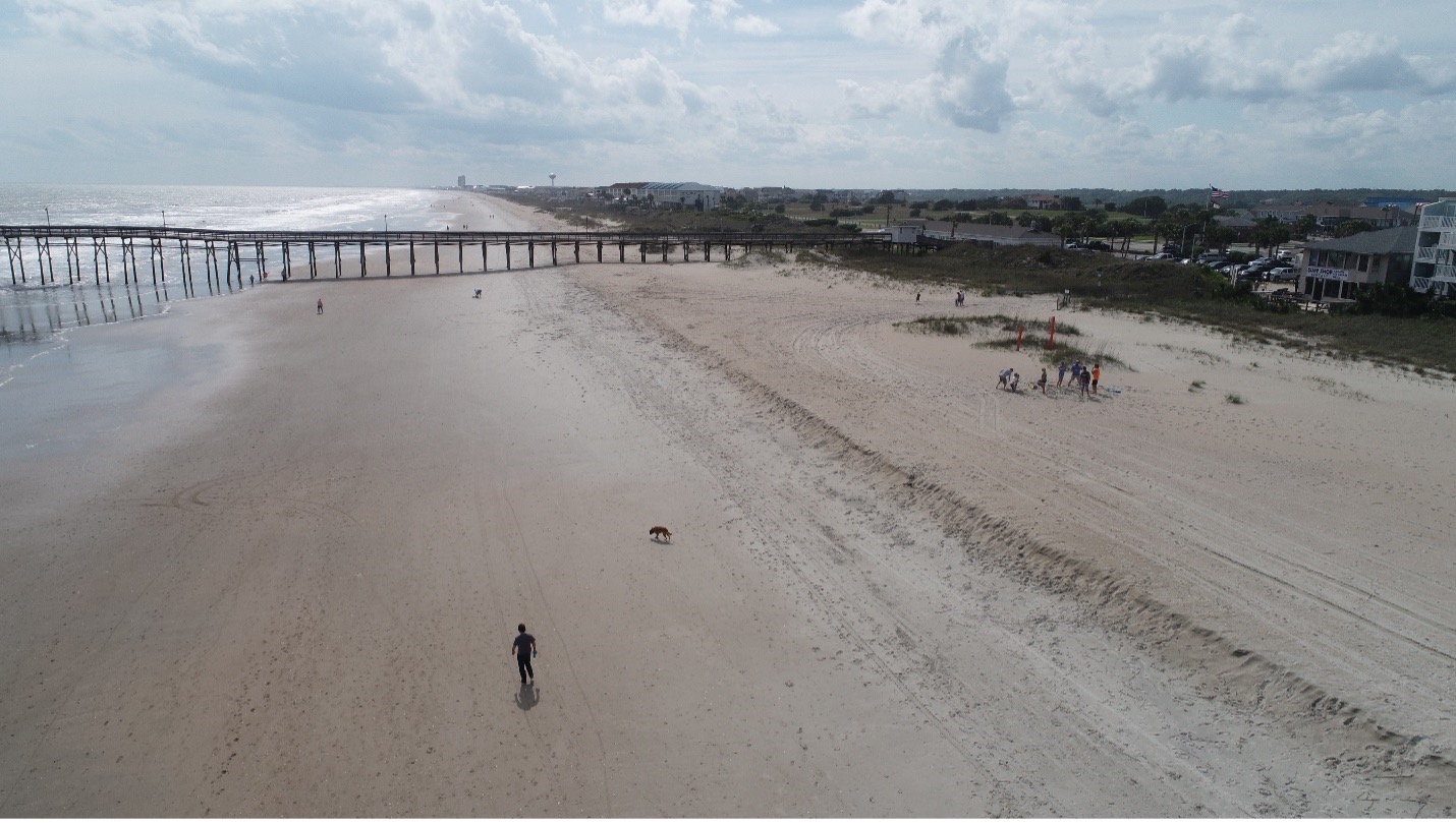
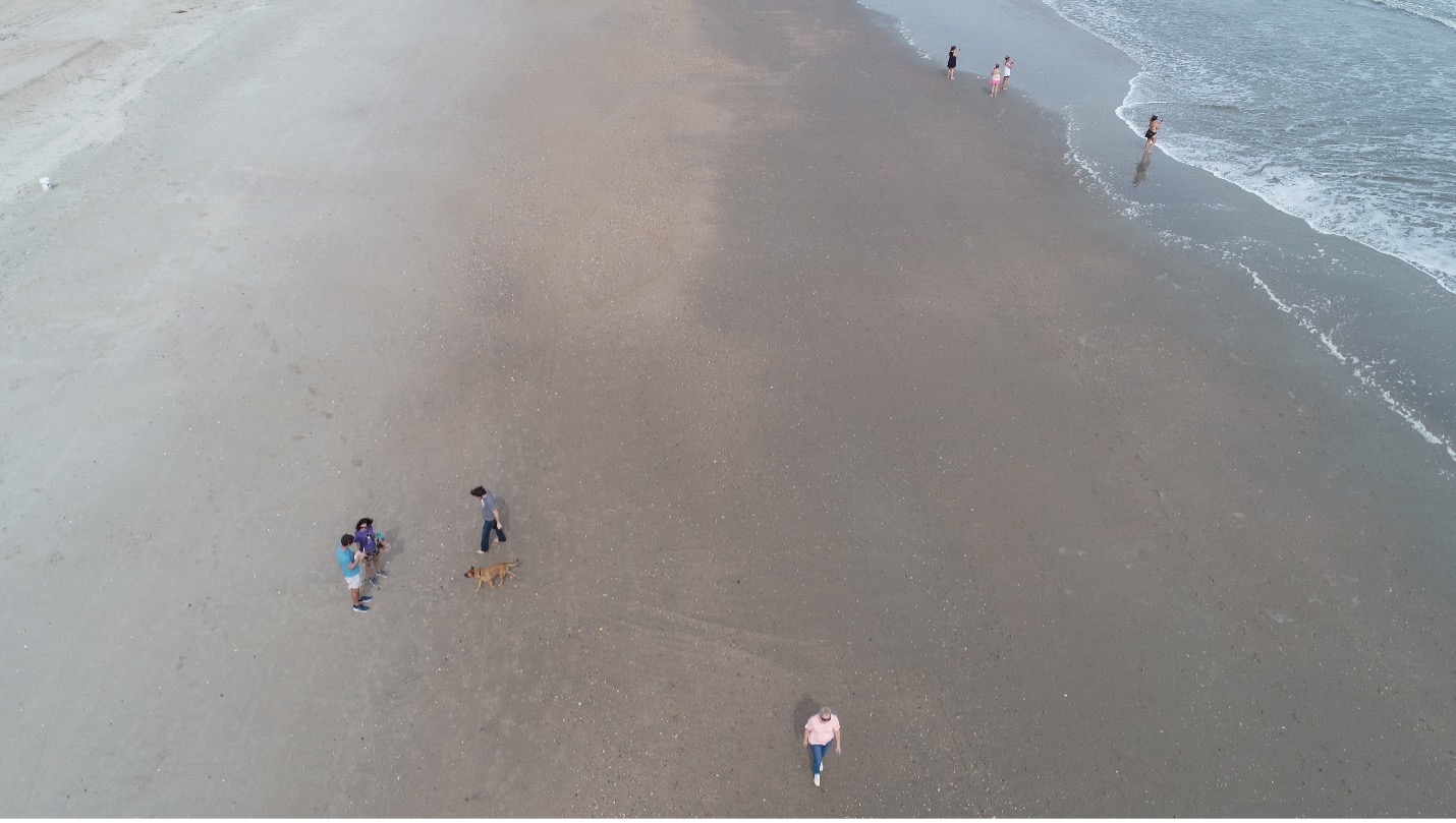
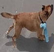
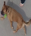
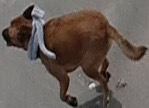
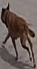
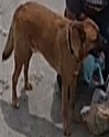
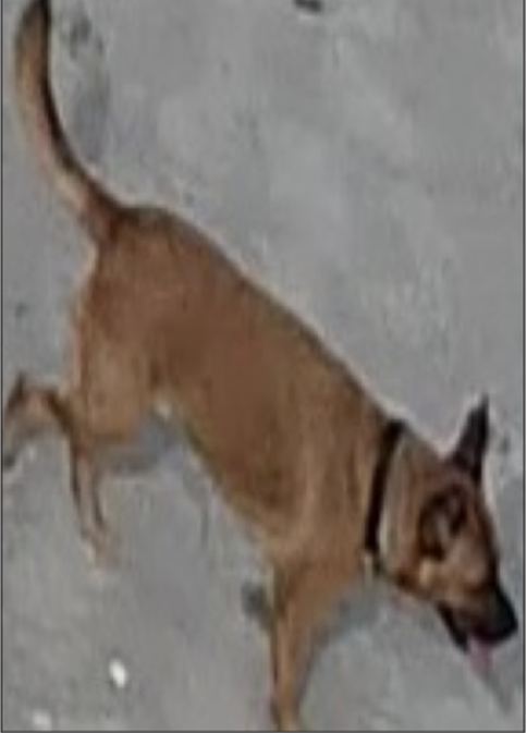
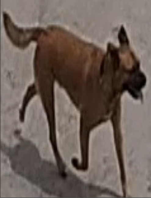
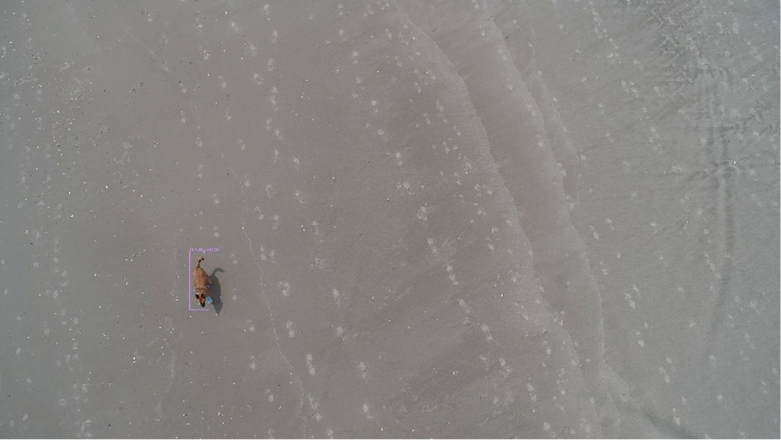
The data comes from aerial photos and videos taken from a drone. The images are a resolution of 5472 by 3078 pixels and contain a dog, Dr. Taco, as he runs around the beach. Here are a few examples (click on a photo to enlarge it):
 |
 |
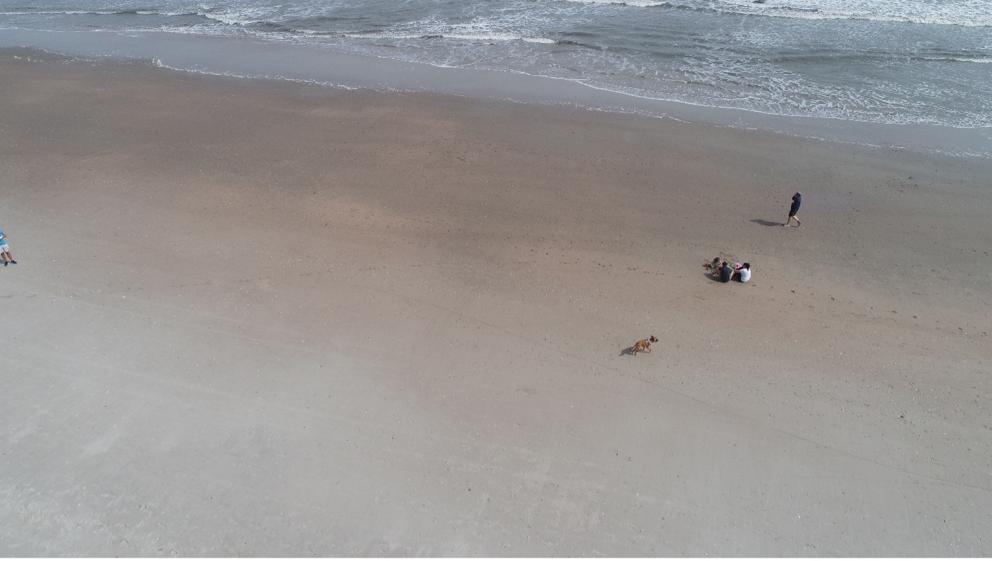 |
Notice that Dr. Taco is wearing a white scarf in figure (c) which may be hard to see. Dr. Taco only fills a small fraction of the large image, which highlights the difficulty of this detection task.
Both Dr. Taco and the drone are constantly moving, making the computer vision task even more difficult because of changing angles, lighting, and the occasional occlusion. In addition, the drone's distance from Dr. Taco is in constant flux and can impact the level of Dr. Taco’s detail granularity, with farther distances resulting in blurrier representations.
There are also slight differences in resolution because some images were taken from the drone picture camera, while other images are extracted from the drone’s video feed, which has a slightly lower resolution (3840 by 2160 pixels).
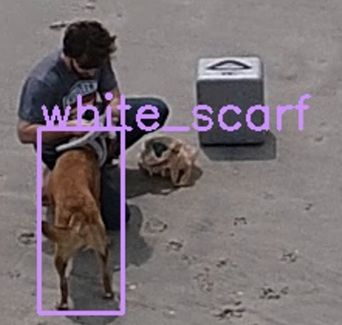
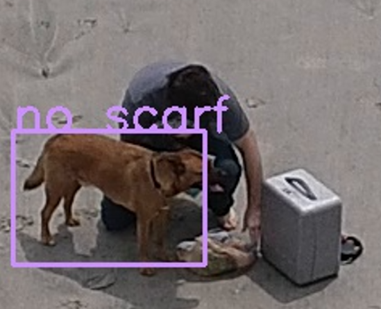
There are four possible outcomes in identifying the color of the scarf around Dr. Taco's neck:
 |
 |
 |
 |

Detecting Dr. Taco’s state is further complicated because of occlusions where Dr.Taco is not fully visible, and edge cases where the scarf is present but not around Dr. taco's neck. In this case, Dr. Taco should be classified as “no scarf.”
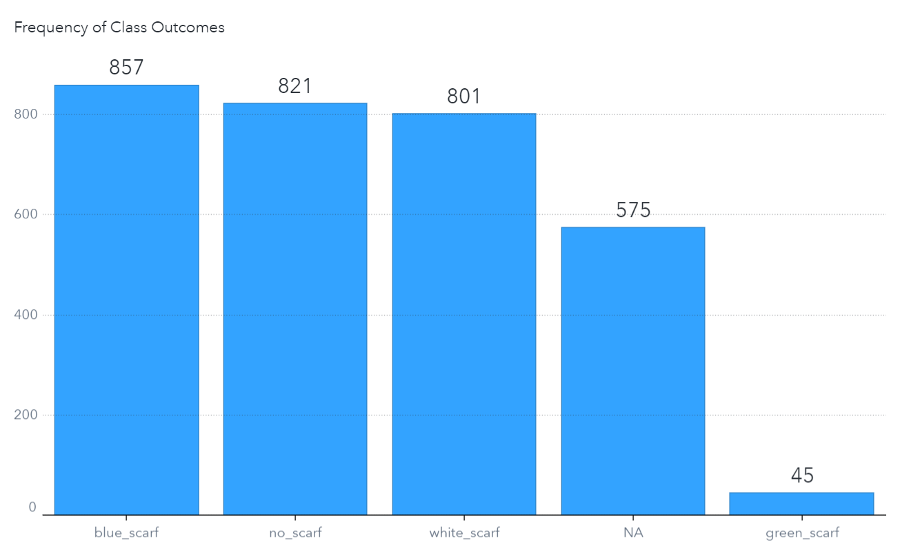
In addition, some state representations are rare. For example, there are only 45 images of Dr. Taco wearing a “green scarf,” whereas there are more representations for the other states:
These challenges led us to create a multi-stage computer vision model where an object detection model first detects Dr. Taco from the images, and a classification model then predicts his state. The location predictions from the object detection model are mapped to the high-resolution version of the image frame, and the new predicted location is extracted. This improves detection accuracy because extractions from the high-resolution image contain a more accurate representation of Dr. Taco. This extraction is then passed to the classifier model to predict Dr. Taco’s state for the classification task. We also use a weighted variable during model training to counteract the imbalance of target (class) distribution which will be explained in more detail.
Multi-stage Computer Vision pipeline
1. Object Detection model
Data preparation
We begin data preparation for our object detection model by labeling the images, meaning we draw a bounding box around Dr. Taco. SAS is developing an annotation tool for image labeling, so at the time of this project, we leveraged LabelImg - an open-source tool for labelling our images. Once images are labeled, the tool generates an XML file for each image, that contains bounding box coordinates of the object that was labeled (in this case, Dr. Taco) and other relevant metadata. These XML files and the image files will be used as training data for building our object detection model.
The SAS DLPy package offers an easy way of merging XML files and the image files to create the training table for our object detection model. Refer to this article to learn how to use DLPy for creating the training table.
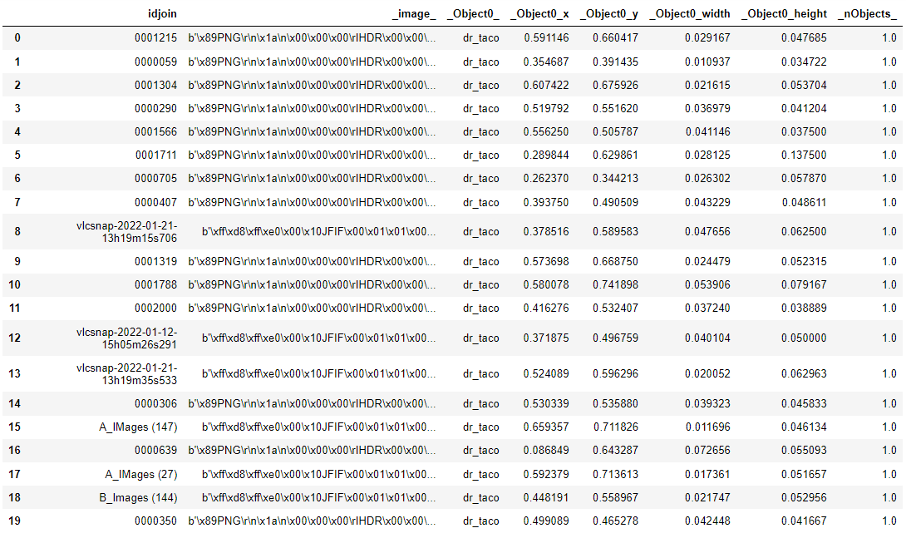
The merged training table contains information where each row corresponds to an image file and the bounding box coordinates of Dr. Taco in that image, as shown below:
We have resized the training images for our object detection model to 416 by 416. Resizing the images to a lower resolution enables transfer learning because many publicly available model weights are trained on 416 by 416 images. This helps us leverage the existing pre-trained model weights instead of creating our model from scratch. Resizing also reduces the prohibitive computational burden accompanying high-resolution imagery training. However, resizing the images to a lower resolution comes with a limitation since we can lose essential details in the image. The loss of granular detail is one of the primary drivers of error.
 |
 |
However, we tackle this problem by mapping model predictions from the resized image back to the original high-resolution image which significantly improves the final predictions. This will be explained later in the article.
Model training and performance
With the flexibility of SAS, users can carry out their Deep Learning tasks either using SAS language or using SAS’s Python API (SWAT) from a Jupyter notebook. The code to perform each of these tasks are the same, except there will be slight differences in syntax of the functions, owing to SAS/Python style of programming. Users can also leverage the SAS DLPy package (for Deep Learning) that serves as a high-level python wrapper for SWAT.
For our model training, we leveraged a pre-trained tiny-YOLOv2 object detection model which requires input images to be 416 by 416. We trained the tiny-YOLOv2 on a dataset containing around 2900 images.
We begin with a few modifications to the existing model structure, to better suit our data. We remove the model’s original detection layer, add a batch normalization layer, a convolution layer, a new detection layer, and we have the model apply random horizontal and vertical flips every mini-batch.
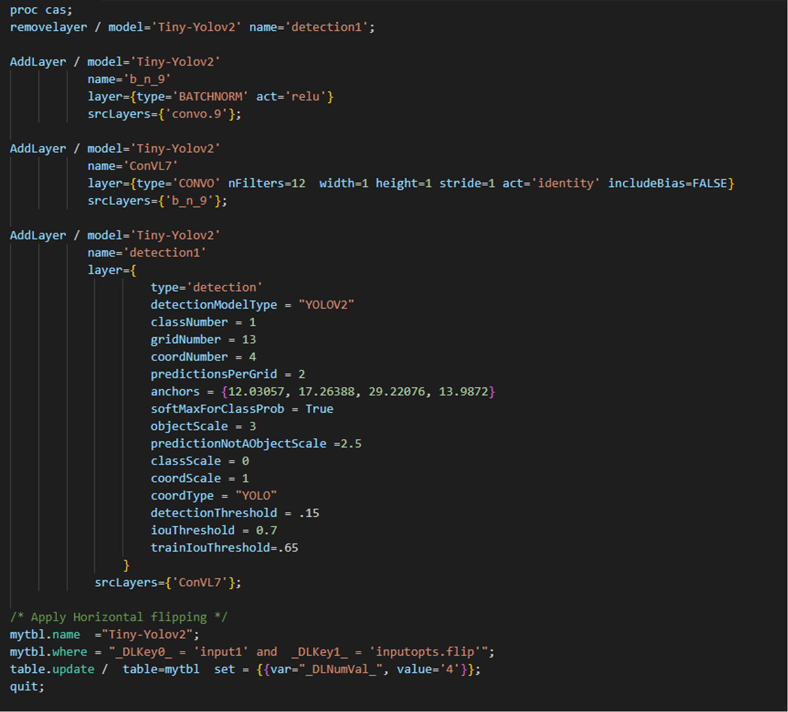 SAS CODE SAS CODE |
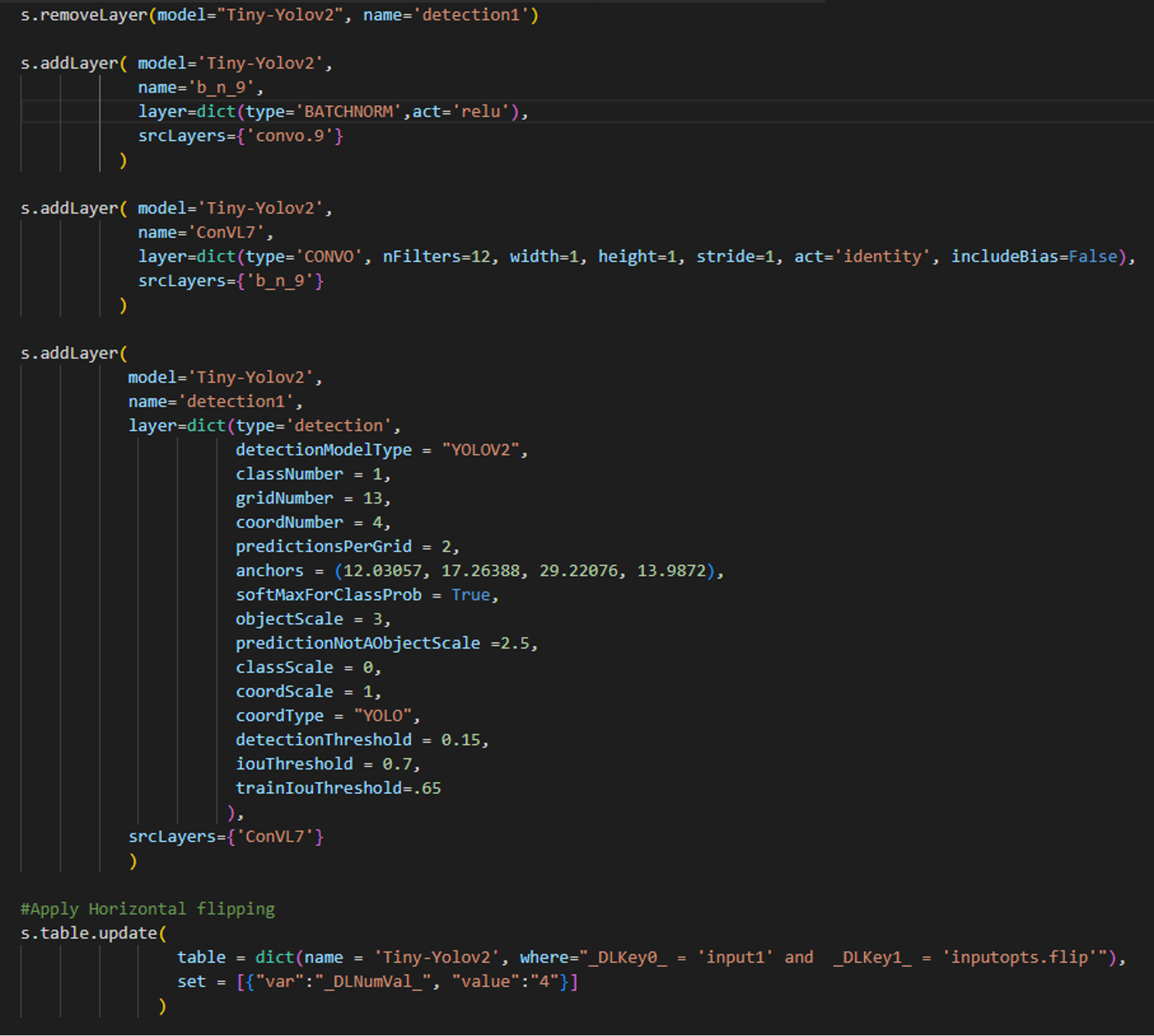 PYTHON-SWAT CODE PYTHON-SWAT CODE |
Irrespective of the language used, the same CAS action is invoked behind the scenes in order to perform a particular task. In the above example code, both languages invoke the same CAS action “addLayer”“” with similar parameters, for adding new layers to the existing model architecture The same approach can be followed for carrying out other analytical steps using the language of preference.
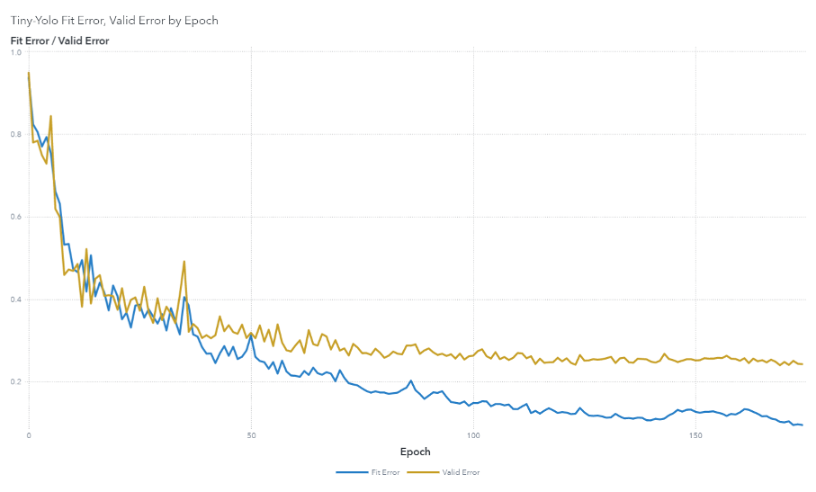
After defining the model architecture, we perform model training using the “dlTrain” action. The input to the model is the training image data while the output is the columns from the object detection table we created earlier using DLPy. We used solveBlackBox action to determine the optimal hyperparameters for our model. See this YouTube video for more details on how to autotune your deep learning models.
The model's performance on the training and validation data is graphed in an iteration plot:
Once the model is trained, our next step is to map the low-resolution location predictions to the high-resolution image frames.
Mapping low-resolution predictions back to high-resolution images
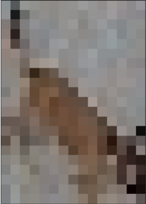
During model inferencing, the YOLO model outputs bounding box predictions of Dr. Taco for each image with a confidence score. However, these are localization predictions for the resized 416 by 416 images. Cropping out these predictions from the resized image might output a pixelated version of Dr. Taco:
 |
 |
Therefore, we need to map these low-resolution predictions back to original high-resolution images to extract a more discernible image of Dr. Taco.
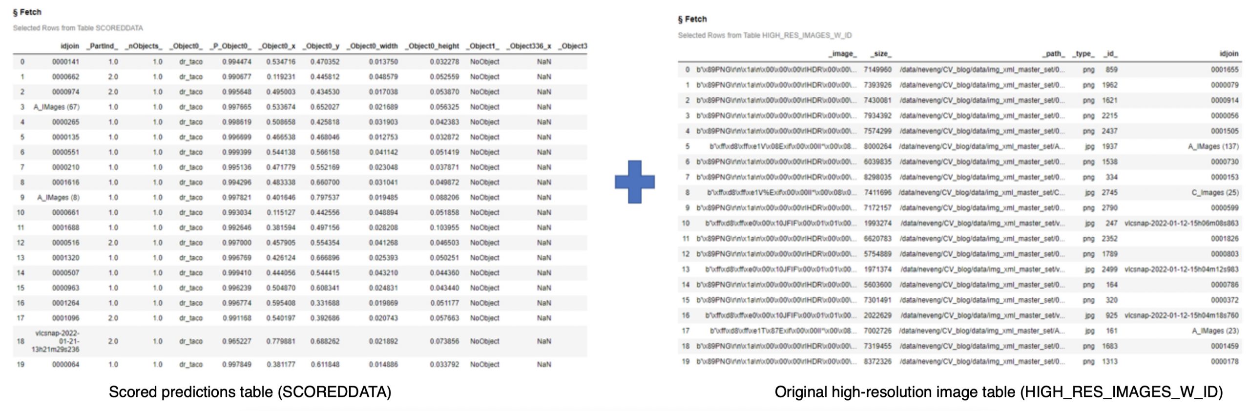
To do this, we merge the original high-resolution image table with the scored predictions table. Since predictions from the scored table are in YOLO format, they are already in a normalized coordinate scale between 0 and 1, hence they can be mapped directly to high-resolution images without any coordinate recalculations. However, if these predicted bounding box coordinates were in COCO/RECT format, new coordinates need to be recalculated in order to do the mapping.
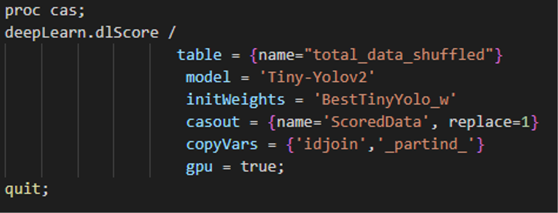
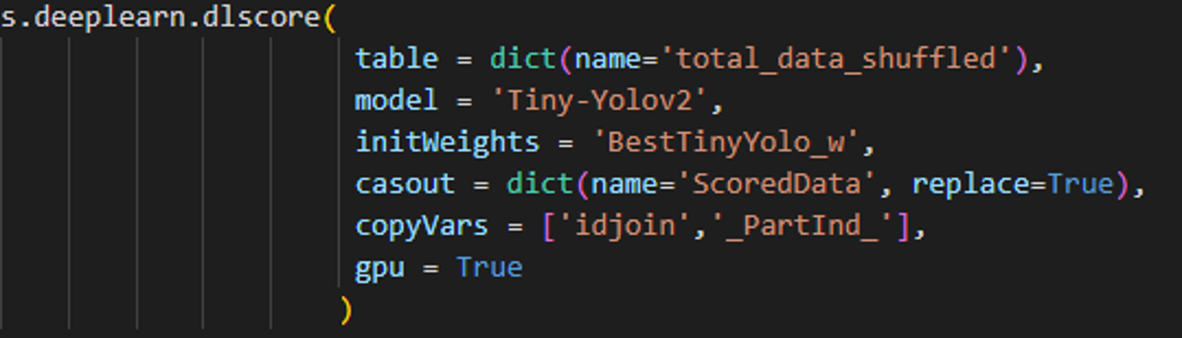
To begin, we perform inferencing (score) on the data using dlScore. The tiny-YOLOv2 model predicts where Dr. Taco is in the image and estimates the size of the bounding box to place around the predicted location. The CASOUT= option specifies the name of the scored dataset containing Dr. Taco's estimated locations and the size of the bounding box.
 SAS CODE SAS CODE |
 PYTHON-SWAT CODE PYTHON-SWAT CODE |
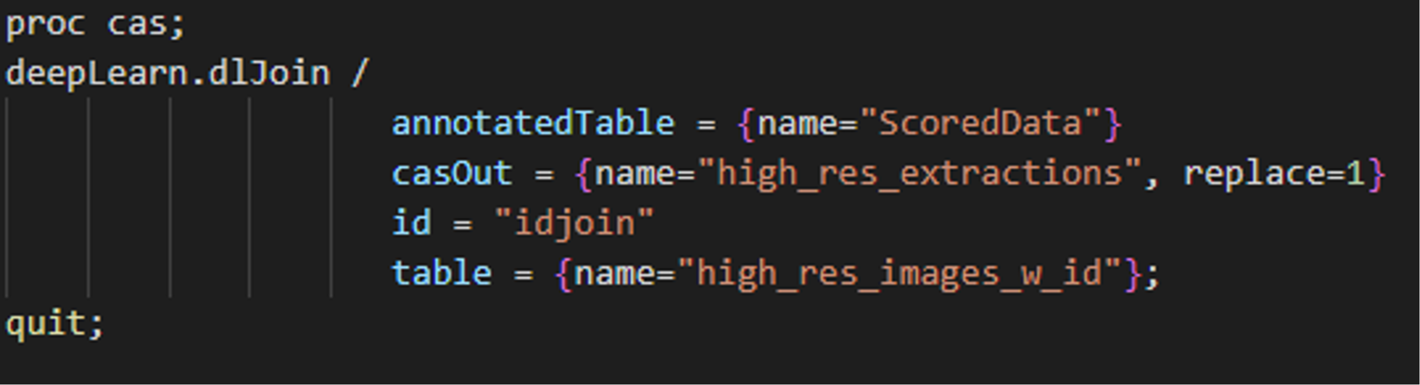
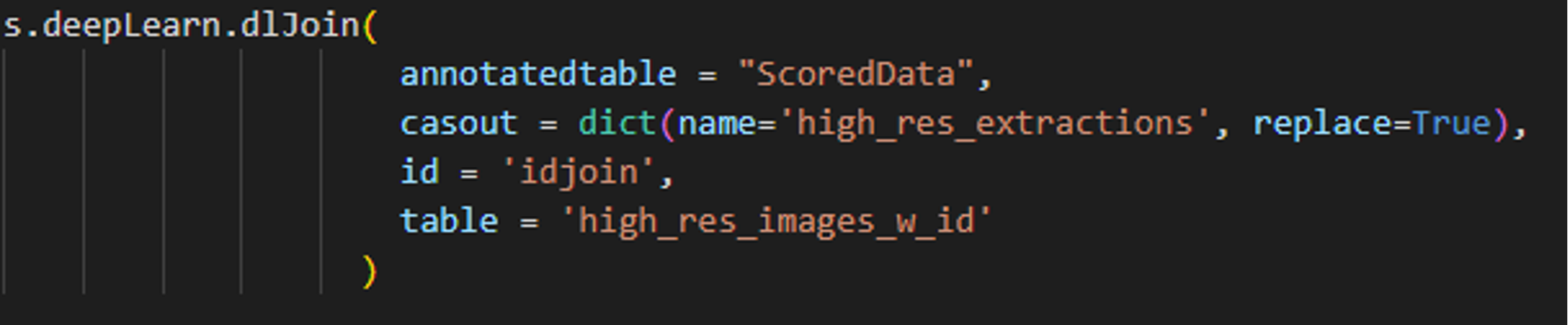
Now, we map our resized localization predictions by joining the scored table with the high-resolution image table based on the common column ‘idjoin’:
 SAS CODE SAS CODE |
 PYTHON-SWAT CODE PYTHON-SWAT CODE |
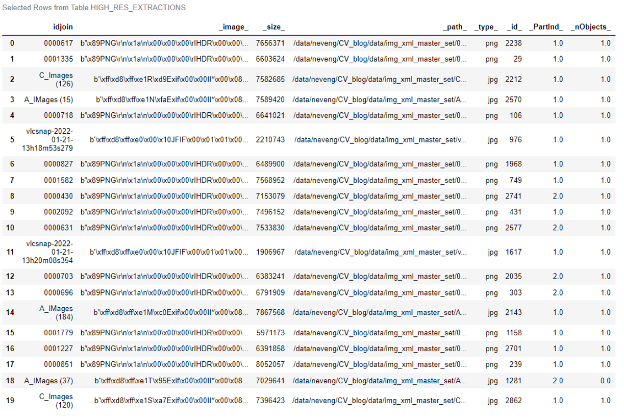
The merged table “HIGH_RES_EXTRACTIONS” now contains the mapped high-resolution localization predictions:
The mapped high-resolution predictions can now be extracted from the merged table using the “extractDetectedObjects” CAS action.
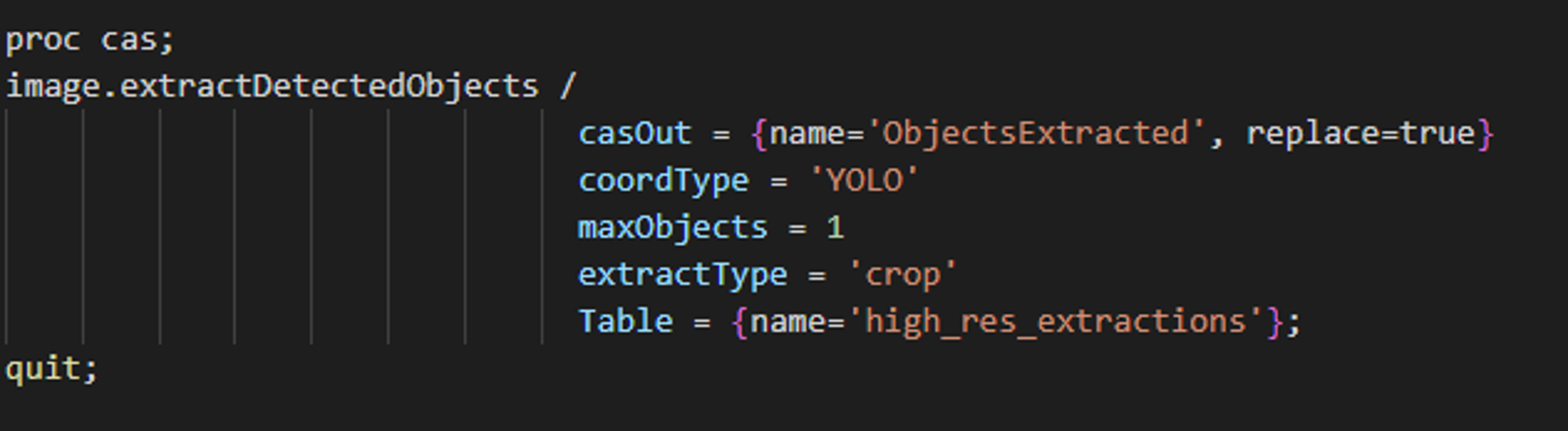 SAS CODE SAS CODE |
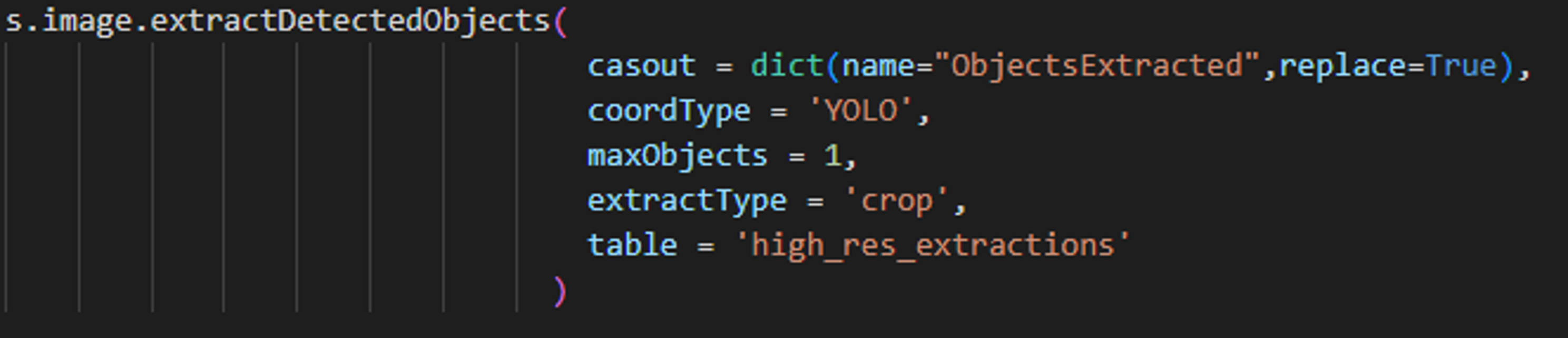 PYTHON-SWAT CODE PYTHON-SWAT CODE |
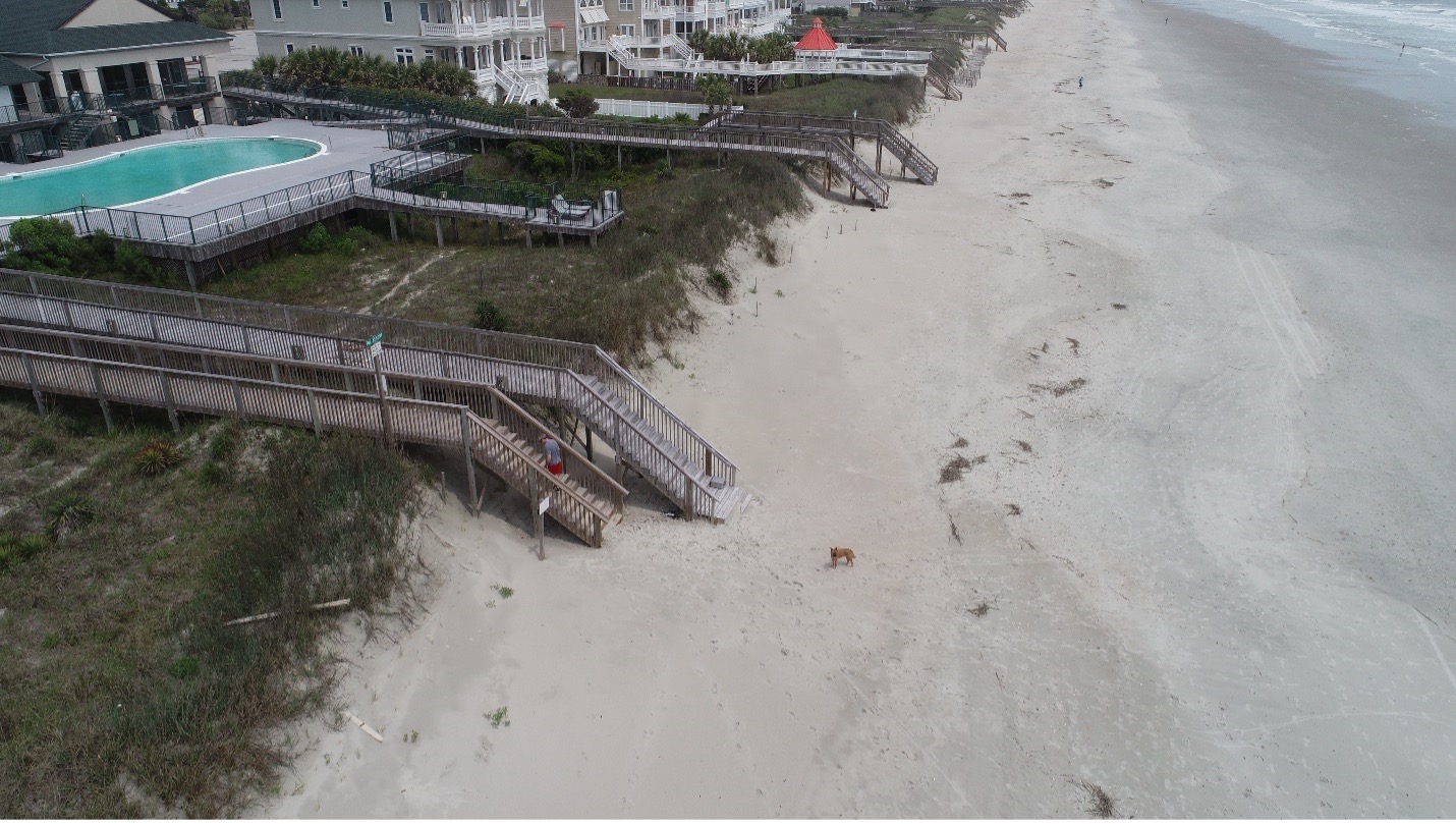
The high-resolution crops of Dr.Taco are now saved to “ObjectsExtracted” table. These images will now be fed into an image classification model for detecting the color of scarf around Dr. Taco’s neck.
 |
 |
2. Image Classification
Data preparation
To prepare our training data for the classifier model, images need to be categorized into folders with appropriate labels. We have four categories of scarf types for Dr. Taco – green scarf, blue scarf, white scarf and no scarf. In addition, we created a fifth class called “NA” which denotes extractions derived from the YOLO model that does not include Dr. Taco. For example, patches of sand. Including NAs as a class allows the classifier model to correct mistakes made by the localization model (YOLO). Hence, the high-resolution crops of Dr. Taco and the cropped patches without Dr. Taco are segmented into five folders with the following class distribution:
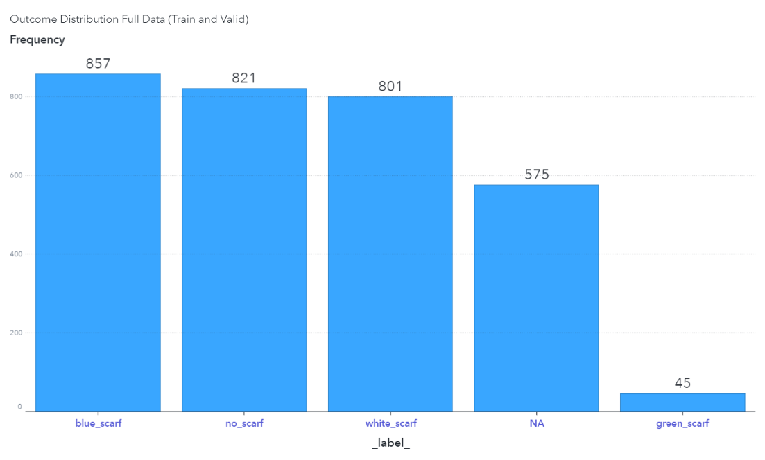
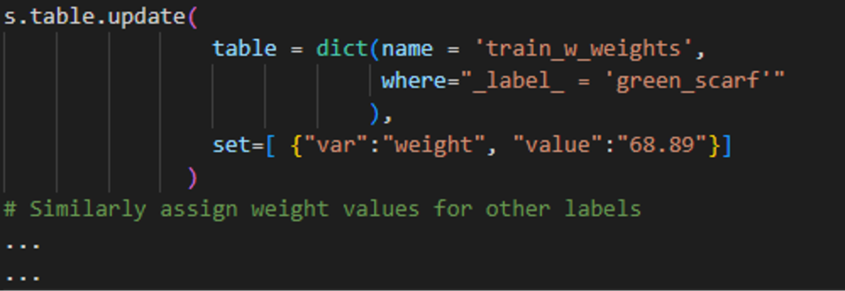
Notice the “green_scarf” label has a smaller representation of images within the training set as compared to the other labels. Rare classes can sometimes be difficult to detect and we address this issue by assigning a weight variable to the training dataset The weight variable is added as a new column to the input image table where the value for each label equals the inverse of the sample priors. That is, 1/relative frequency of that class label in the dataset. For example, there are 36 instances of Dr. Taco wearing the green scarf out of 2,480 in the training data, which is a relative frequency of approximately 1.45%. The weight value assigned to the green scarf outcome is therefore (1 / .0145), or 68.89. This variable can be added to the training table as follows:
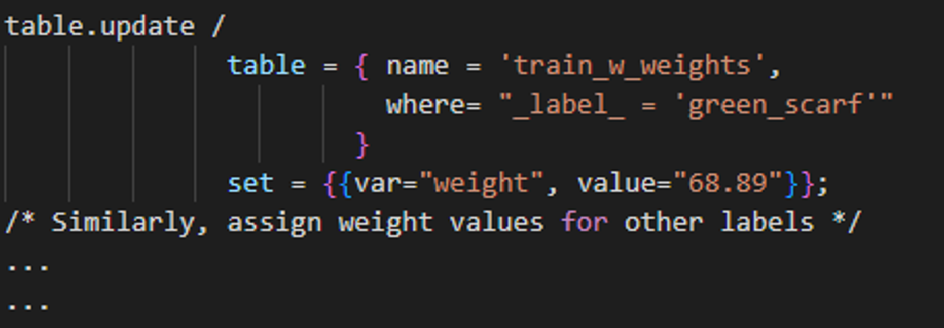 SAS CODE SAS CODE |
 PYTHON-SWAT CODE PYTHON-SWAT CODE |
The updated training table now has a new column added for the weights variable:

Model training and performance
For classification, we tested several classifier model architectures such as VGG15, ResNet50, etc. The ResNet50 model yielded the best performance among all the architectures. Therefore, we went ahead with using the pre-trained ResNet50 model as our image classifier. The ResNet model expects input images to be 224 by 224 pixels, hence we resized our images before training the model.
During model training, we specify the weight variable to accommodate the rare class and improve model predictions.
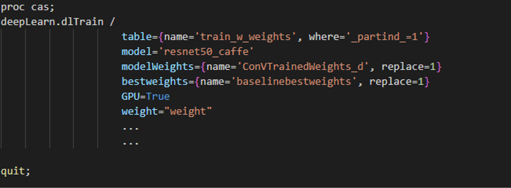 SAS CODE SAS CODE |
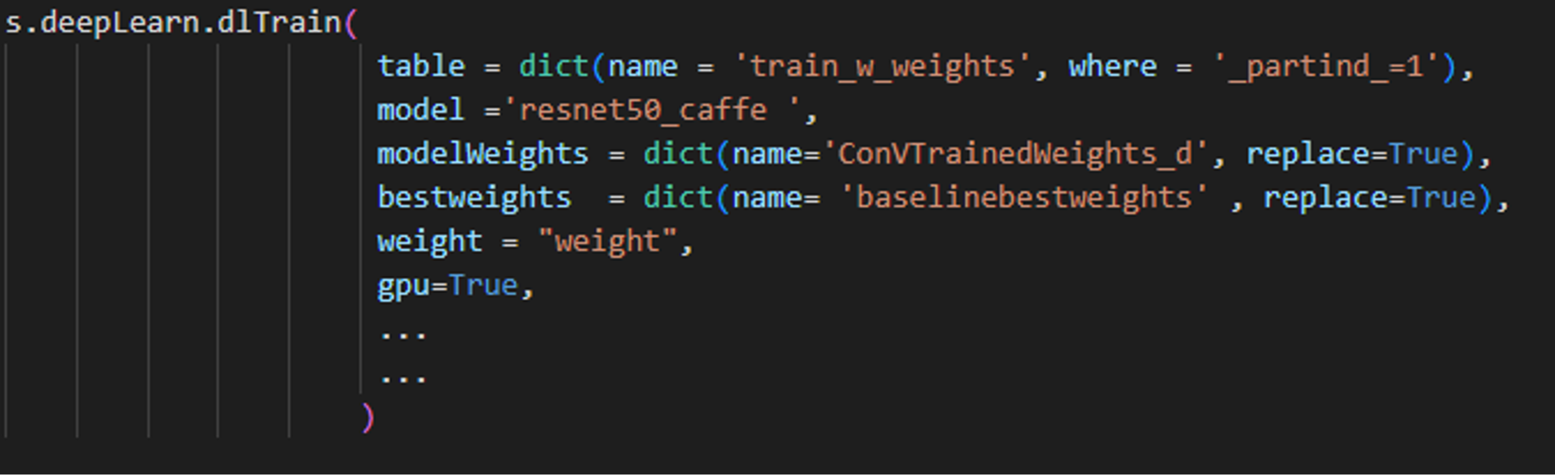 PYTHON-SWAT CODE PYTHON-SWAT CODE |
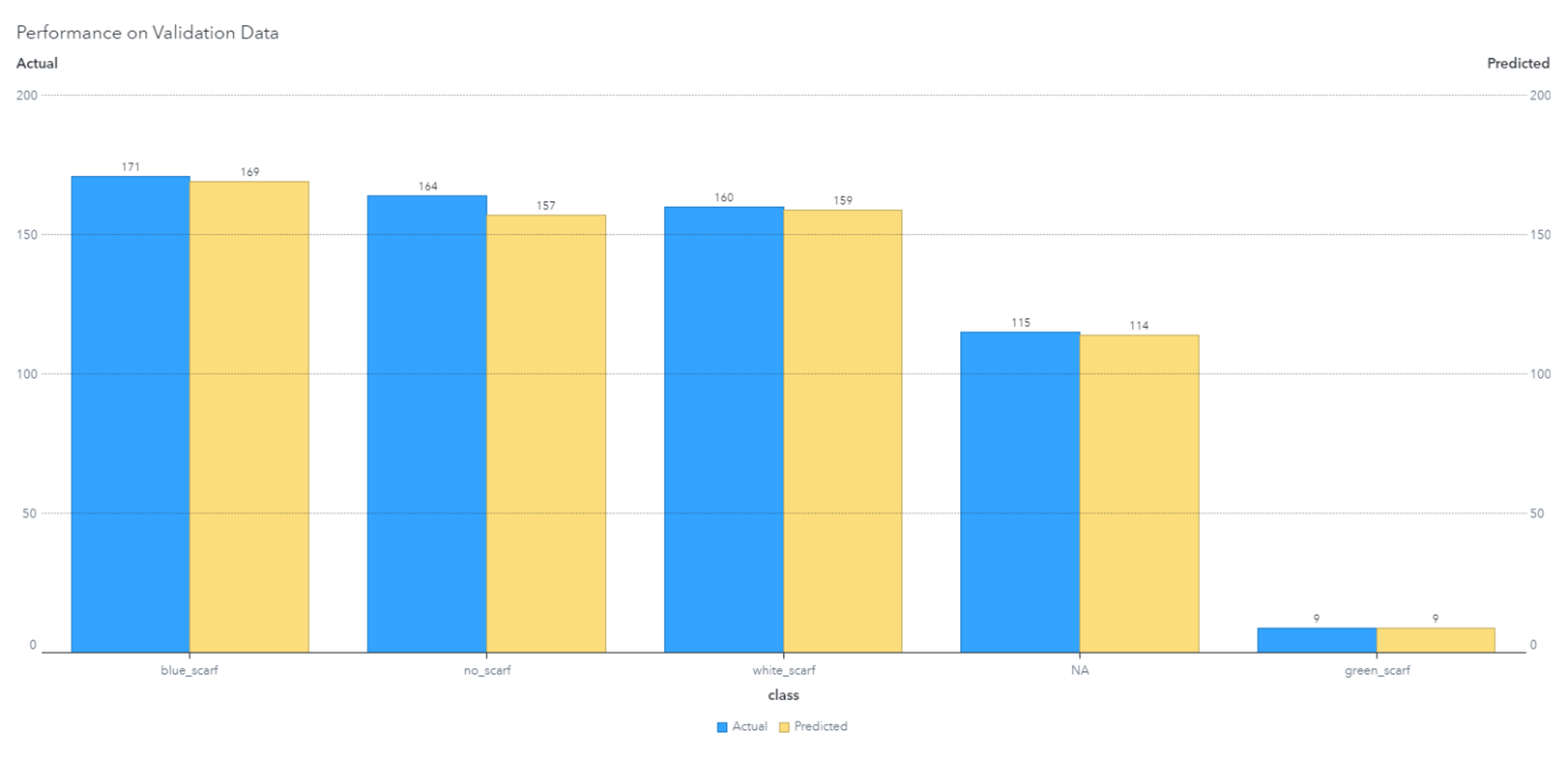
The model's performance on the training and validation data is graphed in an iteration plot:
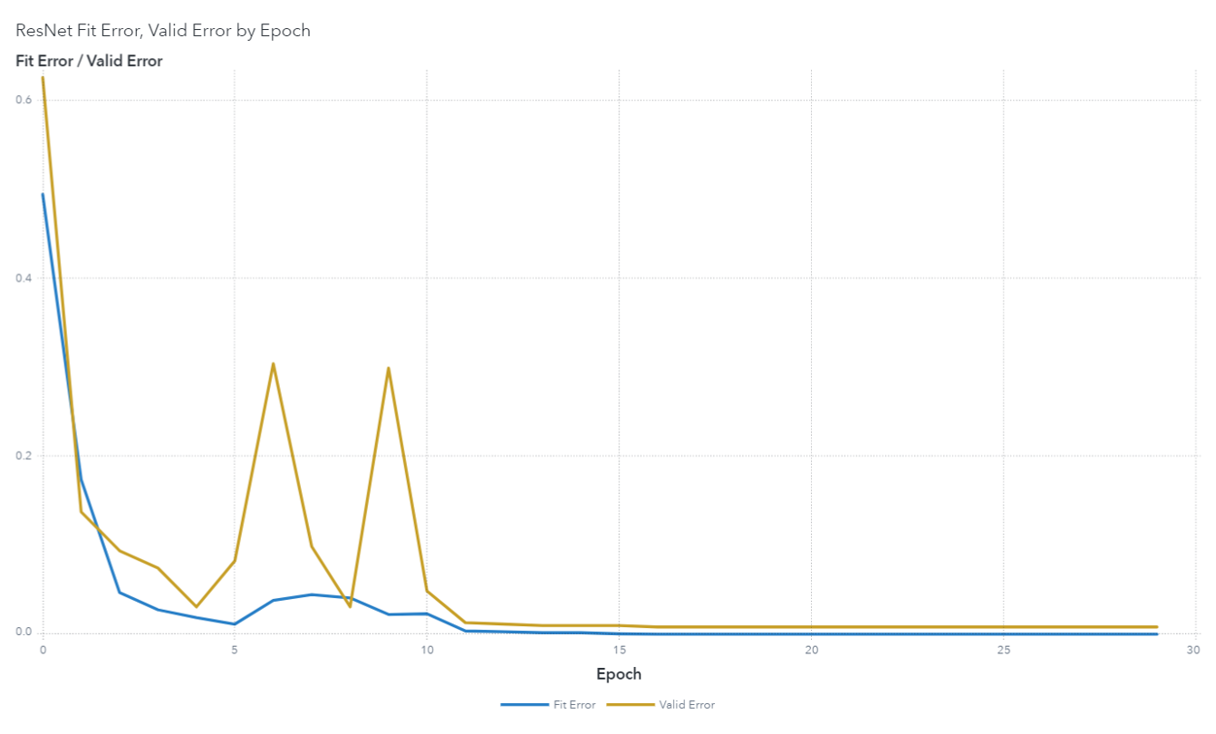
The final predictions of the classifier on the validation set had an accuracy of ~98%.
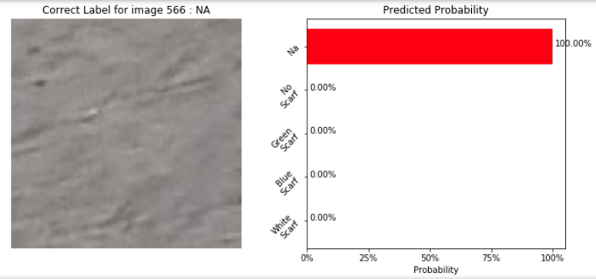
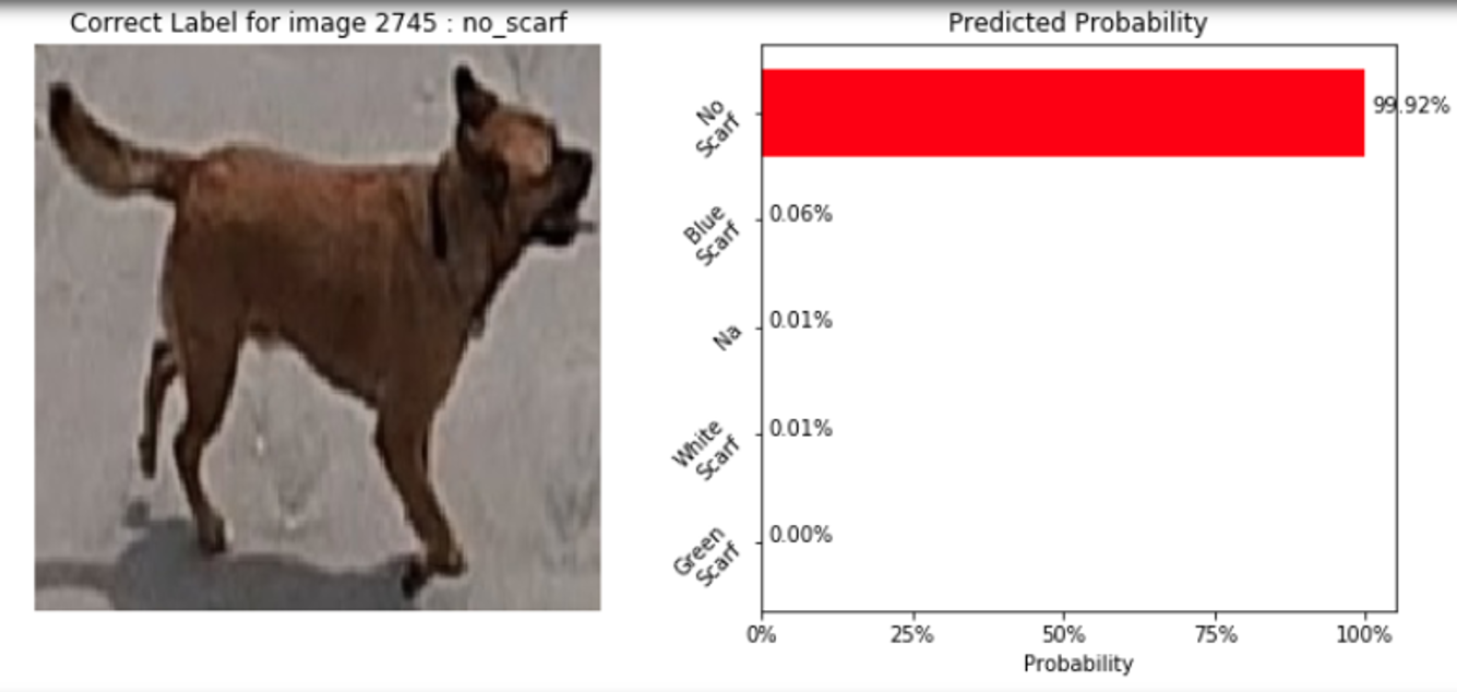
Here are some examples of classifier predictions:
 |
 |
 |
Assessing Model Bias
One of the highlighting features of SAS Viya is the ability to provide model interpretability explanations to understand model predictions. This model interpretability feature helped us to better analyze misclassified images, and also label our data more efficiently.
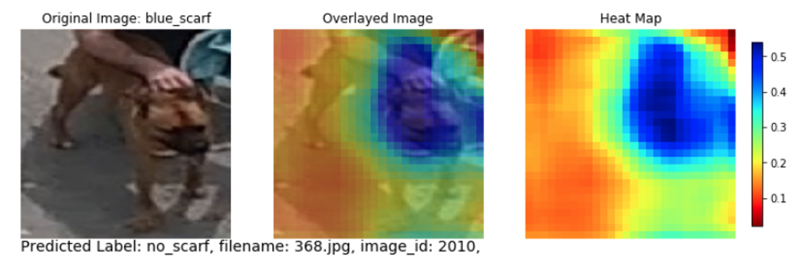
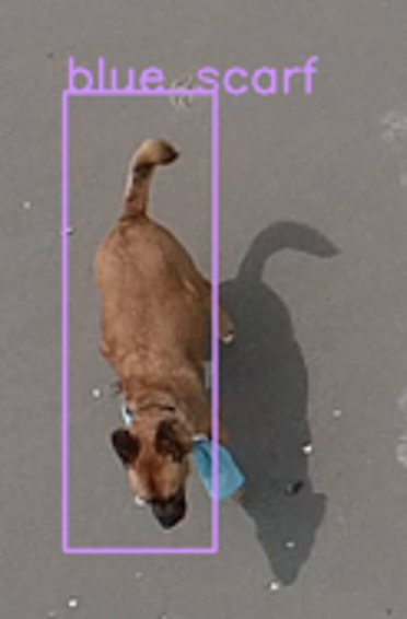
For instance, we wanted to analyze why the model was making an incorrect prediction for one of the images shown below:
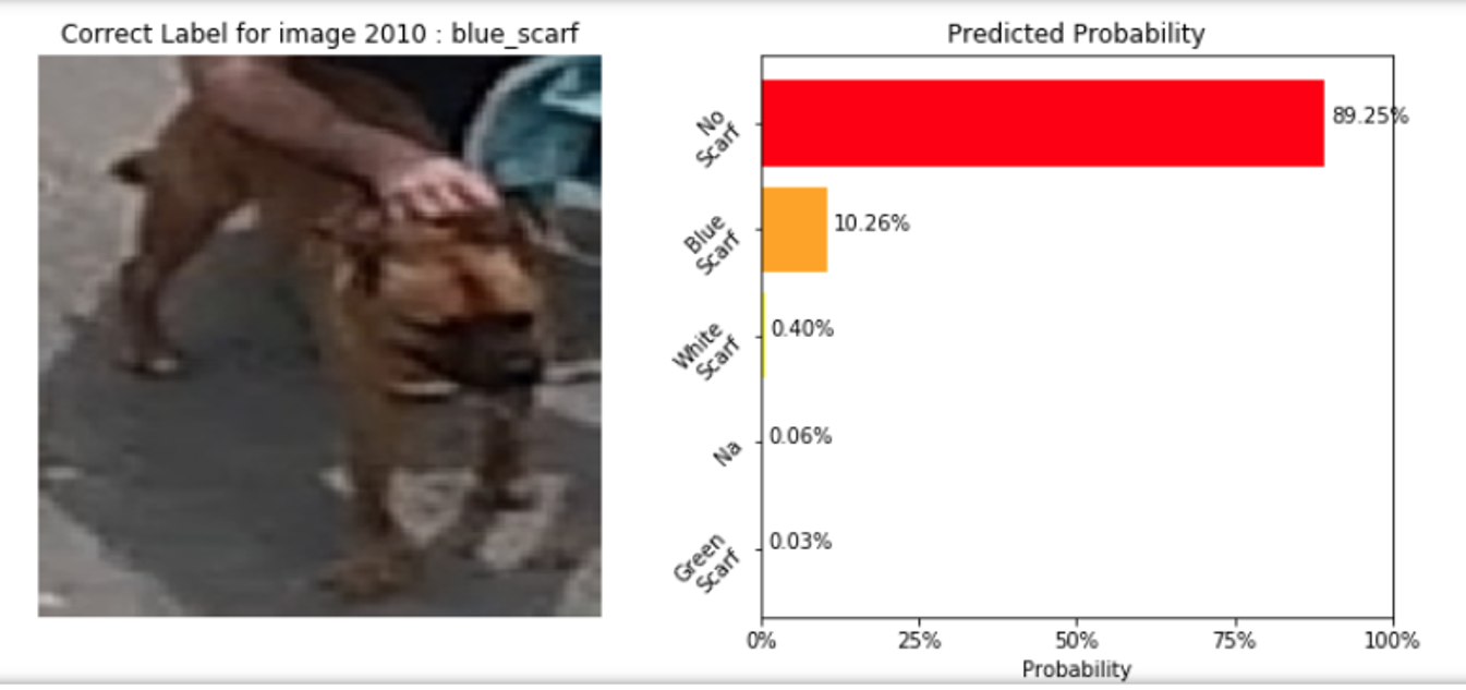
SAS provides heat map explanations with color-coded regions displaying the pixels in an image that the model is focusing on, to make a particular prediction. Plotting the heat map chart for the above image, we found that the blue colored region from the heatmap (see below) is where the model is focusing on, to determine the scarf color around Taco's neck. Since there is no scarf in this region, the model makes a prediction as “no_scarf”, which indeed is right. It turns out that during the initial image labeling process, the above image was incorrectly labeled as “blue_scarf”. This helped us to go back and relabel the image in the right way. Hence, model interpretability played a vital role in our data preparation process.
Conclusion
The use of multi-stage modeling improves accuracy over traditional standalone object detection models. Removing the classification task from the object detection model and assigning the task to a separate classifier allows the model to focus more on object location and box size prediction tasks. Mapping the location coordinates back to the higher resolution version improves the classifier's accuracy. Furthermore, the classifier also provides feedback that can improve localization performance. For instance, when the classifier predicts the class to be "NA," the coordinate predictions can be removed.
Deploying Computer Vision models is now made easier with SAS Viya. The next step in the process deploys the models on a drone using SAS Event Stream Processing (ESP) engine. The follow-up article by Drago Coles details the next steps on using ESP to deploy these Computer Vision models for real-time processing. Below are a few examples of real-time inferencing on individual image frames from SAS ESP:
 |
 |
 |
 |
 |
 |