Neural networks, particularly convolutional neural networks, have become more and more popular in the field of computer vision. What are convolutional neural networks and what are they used for?
Recall from my earlier blog that a computer sees an image as an ordered set of pixels.
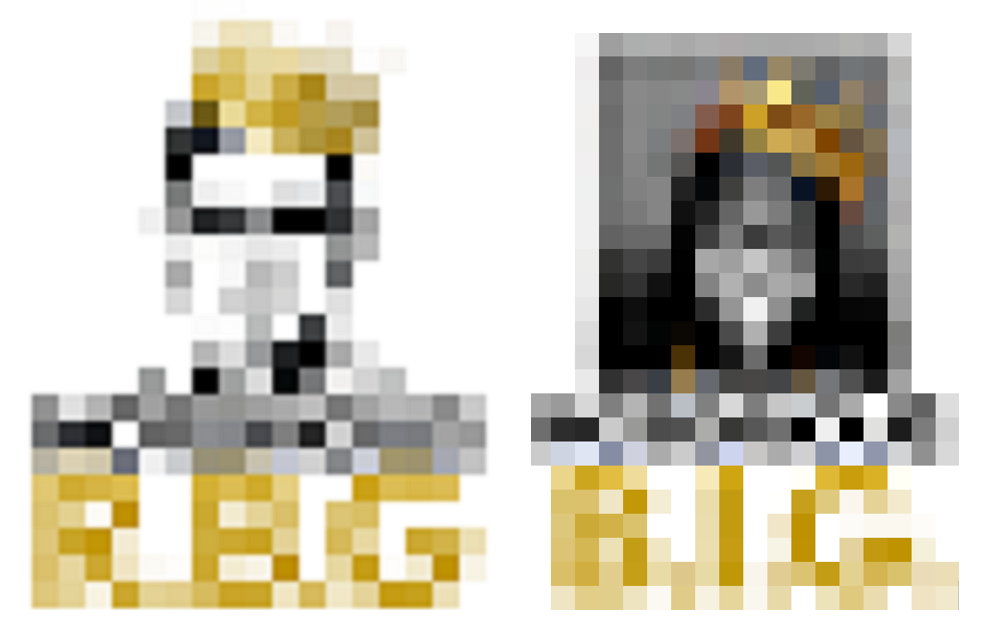
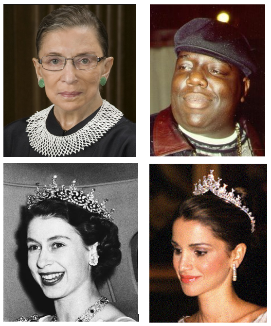
We recall the notorious RGB = red, green, blue (which is NOT the Notorious R.B.G., nor the Notorious B.I.G., so please don’t get confused).
For RGB we have:
- R = red
- G = green
- B = blue
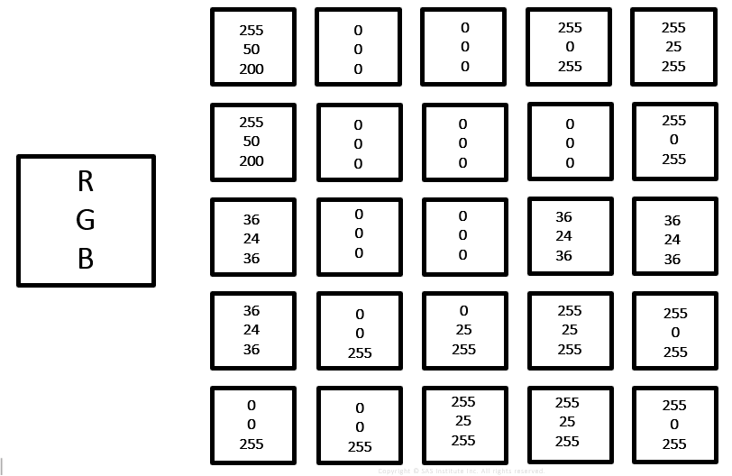
Where each pixel is represented by three numbers from 0 to 255, giving the intensity of red, green or blue.
Here is what 5 pixels by 5 pixels might look like.
But let’s say we have 24 x 24 pixels (as shown in my Notorious RBG and Notorious BIG pictures above), for a total of 576 pixels. Times 3 numbers (R, G, and B) for each pixel, equals 1,728 input numbers. That is a lot of inputs and we can see that in real life we would want to start with more pixels than 24 by 24.
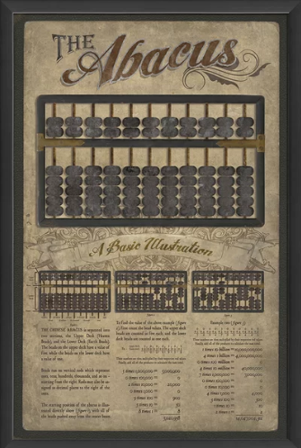
If we had 240 pixels by 240 pixels we would have a total of 57,600 pixels. Times three numbers (R, B, and G channels) equals 172,800 inputs. Color images commonly have over 30 million pixels per channel. Quickly we understand why neural networks were not feasible back in the days of the abacus!
Neural Networks
Let’s quickly review neural networks.
Neural networks are universal approximators. This means that with enough neurons and time, a neural network can model any input/output relationship, to any degree of precision.
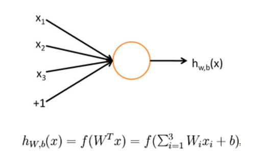
A standard feed forward neural network receives an input (vector) and feeds it forward through hidden layers to an output. SAS PROC NNET, for example, trains a multilayer perceptron neural network. As the name “multilayer” implies, there are multiple layers. Below we see the inputs (features), one hidden layer and the output (response, target). Each neuron is simply a mathematical function.
The hidden units include a default link function (an activation function), which may be the sigmoid function, hyperbolic tangent, ReLU, ELU, etc.
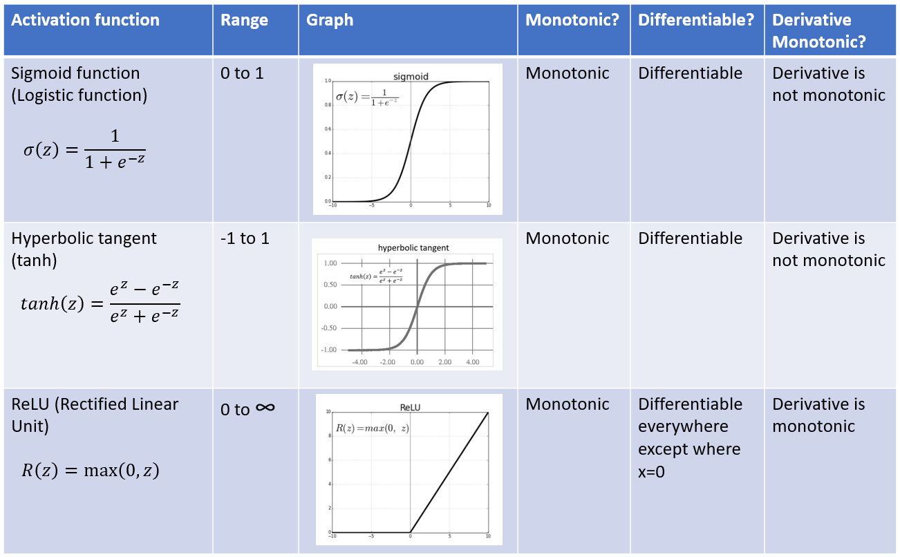
Note: A single neuron with sigmoid function corresponds exactly to the input-output mapping defined by logistic regression. So one way to conceptualize multilayer perceptrons is as regressions on hidden units, with the hidden units themselves conceptualized as regressions on the original inputs.
ReLU is commonly used in CNNs. It replaces all negative pixel values in the feature map by zero. All positive values retain their same value.
Deep Learning is More Than Just Lots of Layers
It can be tempting to think of deep learning as just more layers, like a Smith Island Cake (Maryland’s state dessert, by the way). Although deep learning methods commonly do include many layers, there is more to deep learning than just more layers.

Among other things, deep learning methods commonly include (largely from SAS Education Deep Learning Using SAS Software course by Robert Blanchard and Chip Wells):
- Activation functions resistant to saturation. For example, Rectified Linear Transformation (ReLU) and Exponential Linear Activation Transformation (ELU) are more resistant to saturation than sigmoid or hyperbolic tangent functions.
- Normalized initializations of weights where variance of the hidden weights is a function of the amount of incoming information, e.g.,
- Xavier initialization
- MSRA
- MSRA2
- New regularization techniques, e.g.,
- Dropout
- Batch normalization
- Fast moving gradient-based optimizations, e.g.,
- Stochastic gradient descent
- Adam, AdaMax
- Innovations computing, e.g.,
- Parallel processing
- GPUs
Convolutional neural networks are designed to be more efficient than traditional neural networks. They do this in part by extracting features from in an image. An example of a feature might be an edge.
As described in the SAS documentation, “convolution is the process of analyzing an input image, represented as an array of pixel values, by iteratively sliding (convolving) a smaller matrix (filter) across the input image, while performing elementwise calculations to compute an output matrix of image features.” You can think of a convolution as a sliding window function applied to a matrix.
The Layers
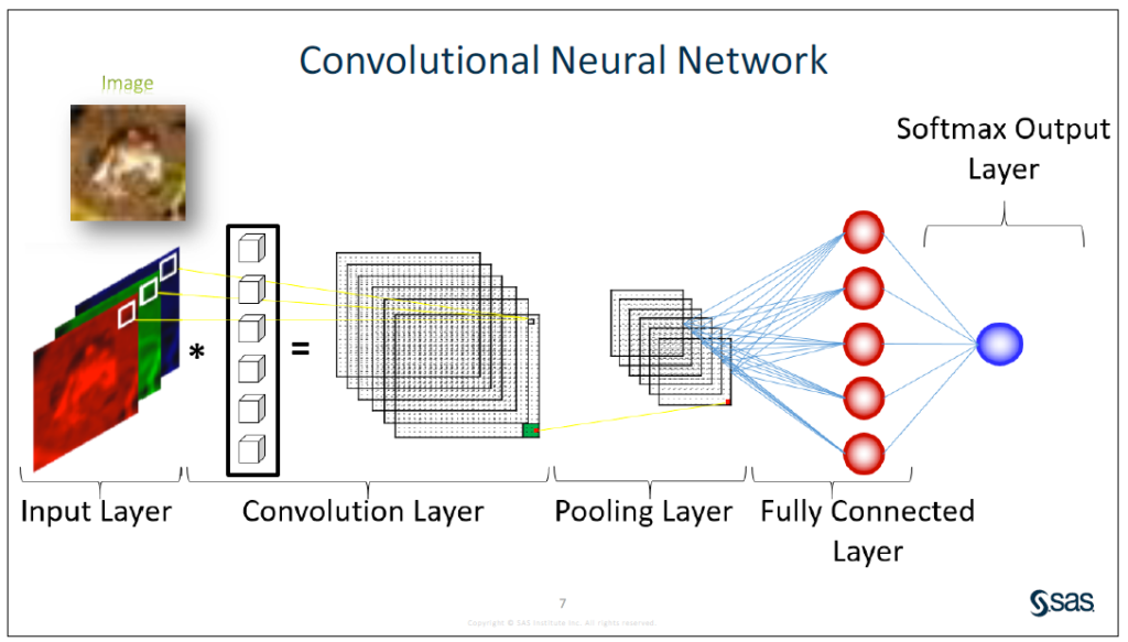
Convolutional neural networks (CNNs) usually include at least an input layer, convolution layers, pooling layers, and an output layer. An image is read into the input layer as a matrix of numbers (1 layer for black and white, 3 layers or “channels for color”: R, G, B). An output comes out with a score associated with possible labels for the image (or a portion of the image). In facial recognition software, for example, the face labels might be Ruth Bader Ginsburg, Christopher George Latore Wallace, Elizabeth Alexandra Mary Windsor or Rania Al-Abdullah.
A couple of diagrams below attempt to provide a simplified illustration of the convolutional neural network process.
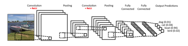
Source: https://ujjwalkarn.me/2016/08/11/intuitive-explanation-convnets/
SAS Deep Learning supports typical convolutional neural network layers shown in the table below.
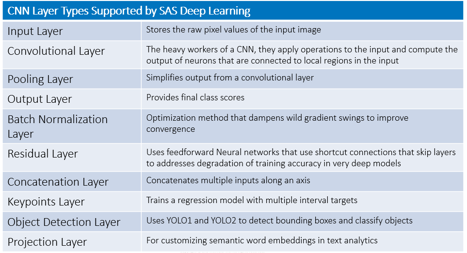
Let me describe a few of these layers. For more examples and details, see the documentation.
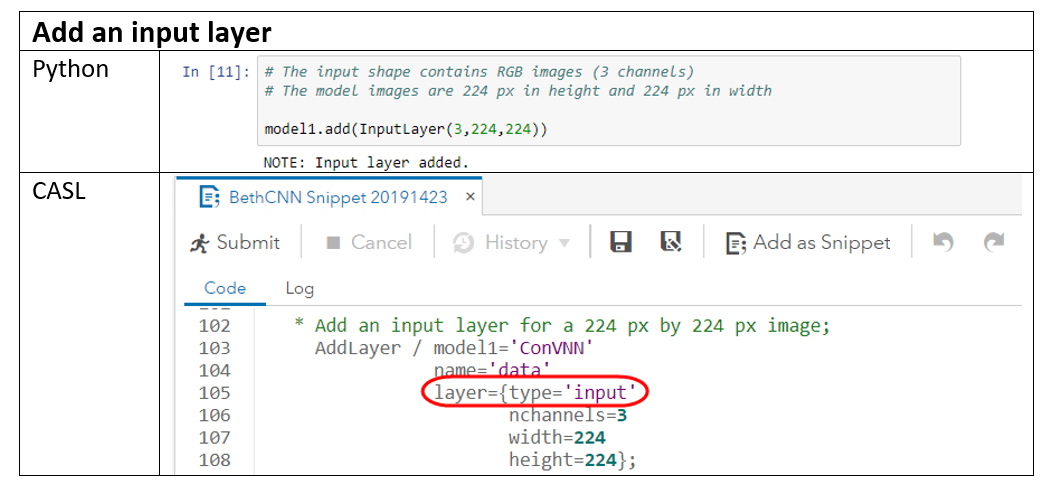
Input Layer stores the raw pixel values of the image. In the sample code below, the input layer has 3 color channels (R, G, B), a height of 224 pixels, and a width of 224 pixels.
Convolution layers are the crux of the convolutional neural network. They use filters to extract features from the input image. A filter is also referred to as a kernel or feature detector. It can be thought of as a sliding window of weights. These weights are learned during training. That is, a CNN “learns” filters that are proficient at detecting certain types of visual features, such as a straight line, a semi-circle, and other image features that may be meaningless to humans, but that are helpful in determining a correct outcome.
Filters usually have small width and height and, of course, they share the same depth as the input. For a color image, the filter depth is 3, for the three color channels of blue, green, and red. For a black and white image, the filter depth is 1.
We slide the filter over the image at a certain stride, and the dot product is computed. Stride is simply the number of pixels we slide over each time we move the window. The dot products create a new matrix called the convolved feature or activation map or feature map.
Filter examples are shown below:

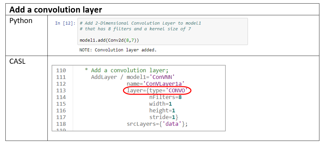
The sample code below adds a 2-dimensional convolution layer with 8 filters and a kernel size of 7.
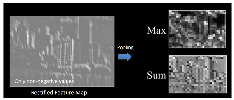
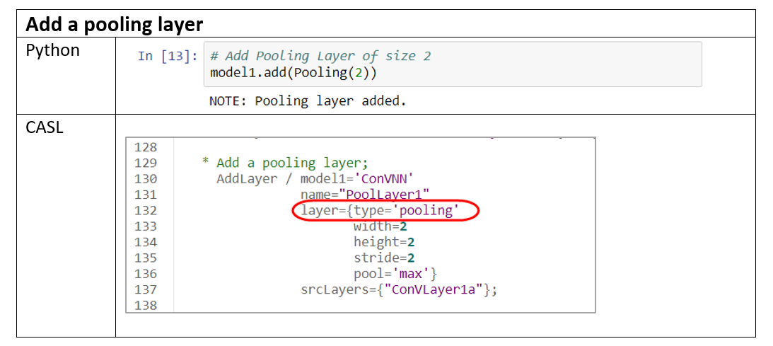
Pooling Layers are commonly placed between successive convolution layers to simplify the output from a convolution layer. A pooling layer downsamples to reduce the dimensions (and thereby reducing computational parameters).
Popular types of pooling include:
- Max pooling (most popular)
- Average pooling
- Sum
- L-2 norm, etc.
The sample code below adds a pooling layer of size 2.
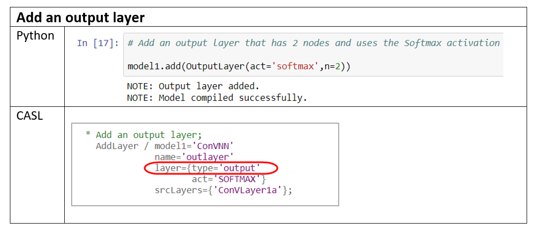
The Output Layer is a fully connected layer that is associated with a particular loss function that computes the prediction error. Being a fully connected layer, the neurons in the output layer connect to all of the activations in the previous layer.
The softmax function takes a vector of scores and transforms it to a vector of values between 0 and 1 that sum to 1. Thus applying softmax as the activation function ensures that the sum of output probabilities from the fully connected layer is 1.
The sample code below adds an output layer that has 2 nodes and uses softmax activation function.
CNNs transform original images to the final class scores layer by layer. The convolution and output layers contain parameters, but the pooling layers do not. Optimization techniques such as stochastic gradient descent or L-BFGS can be used to train and compute the parameters in convolution and fully connected layers.
Why Use Convolutional Neural Networks?
- Traditional forward feed neural networks don’t scale well to full images
- The capacity of CNNs can be controlled by varying their depth and breadth
- CNNs make strong and mostly correct assumptions about the nature of images (namely, stationarity of statistics and locality of pixel dependencies)
- Compared to standard feedforward neural networks with similarly sized layers, CNNs have fewer connections and parameter so they are easier to train and their performance is not much worse
“For a fully connected regular neural network, the number of neurons can be large. Using fully connected architecture, the number of weights can become enormous, and require exceptional amounts of memory and computing resources in order to train the network. CNNs can minimize the number of neurons by taking advantage of the architecture of image inputs. In contrast to fully connected networks, CNNs connect each neuron only to a local region of the input. The dimensions of this local region are defined by the filter size. Using a smaller local region drastically reduces the number of neuron connections and weights when compared to fully connected networks.” –SAS documentation
A Little History
First, a little history. In 2012, Alex Krizhevsky and Ilya Sutskever (students of Geoffrey Hinton at University of Toronto) trained neural networks and won the 2012 ImageNet classification challenge by a huge margin. He got top-five error rates down to only 17 percent!
Krizhevsky and Sutskever trained a neural network with:
- 60 million parameters
- 650,000 neurons
- 5 convolution layers (some followed by max-pooling layers)
- 3 fully connected layers
- 1,000-way softmax
- 5 to 6 days to train on 2 GTX 580 3GB GPUs
They expedited training by using non-saturating neurons and GPUs (graphics processing units).
They reduced classification error dramatically using convolutional neural networks. They won the ILSVRC-2012 competition and achieved a top-5 test error rate of 15 percent compared to 26 percent by the first runner up entry.
In the late 20th century, Yann LeCun and colleagues began developed a convolutional neural network called the LeNet to recognize hand written numbers. “LeNet uses the same weights for the same filter across different locations in the first two layers. This significantly reduces the number of parameters needed to be learned compared to a fully connected neural network. The underlying concept is fairly simple; if a filter that acts like an edge detector is useful in the left corner then it is probably also useful in the right corner.” See Li Yang Ku’s blog.
What Took So Long?
If convolutional neural networks and LeNet emerged in the 1980s, why did they gain so much popularity only more recently?
1. Data
- Millions of labeled images are available now for training neural networks. Data sets available to the public include LabelMe and ImageNet (>15 million labeled high-resolution images in over 22,000 categories).
- Organizations like Tencent, FaceBook, Google, Baidu, and Alibaba have access to hundreds of millions of images for training.
2. Hardware
- Modern hardware let us train multilayer neural networks with millions of observations of training data by exploiting parallel processing
- GPUs
- Highly-optimized implementation of 2D convolution
3. Algorithms
- Algorithm and process improvements let us better train neural networks. Examples include:
- Dropout randomly drops units to prevent co-adapting, to help avoid overfitting
- Improved loss functions
- Bundling: Deep Learning bundles feature detection and classification. Old approaches separated these, for example detecting features with something like the SIFT detector and classifying objects with something like a support vector machine. Bundling lets you train both together allowing better features to be learned from the raw data based on classification result through back propagation.
References and More Information
My blog on Computer Vision: What is It?
CS231n Convolutional Neural Networks for Visual Recognition
Understanding Convolutional Neural Networks for NLP
SAS Education Deep Learning Using SAS Software course by Robert Blanchard and Chip Wells
But what *is* a Neural Network? | Deep learning, chapter 1
The Neural Network Zoo by The Asimov Institute
ImageNet Classification with Deep Convolutional Neural Networks Krizhevsky et al.
SAS DLpy documentation: Deep Learning Technical Concepts
SAS DLpy documentation: Deep Learning Action Set Examples
SAS DLpy documentation: Layers in CNNs
Video Demo: Deep Learning with Python (DLPy) and SAS Viya
Getting started with SAS DLPY
CNNs in SAS VDMML 8.3: Deep Learning Programming Guide


1 Comment
This is an absolutely brilliant blog, very well summarised and really enjoyed reading it!