This is the third post describing a computer vision project I worked on at SAS to identify liver tumors in CT scans. In my previous post I talked about testing different models and hyperparameters for the models. Today, I’ll talk about data processing for image data. If you need to catch up, read my previous posts here.
Somewhere around the halfway point of my project, I realized that I needed to leave my deep learning models alone for a while, so I could come back later with fresh eyes. In the meantime, I wanted to start tackling the pre-processing and post-processing of the data to complete the pipeline on either end of the core model.
The first step in the data processing pipeline is taking the raw image, increasing its contrast through histogram equalization, cropping it to a relevant size, and padding it on all sides by 128 pixels (I’ll explain this in a bit) and generating patches from it. These patches will be used to turn this segmentation task into a classification task.
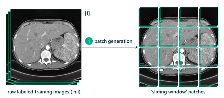
The method I’m using is called the sliding window approach. This approach requires dealing with the 3D CT scans as hundreds of 2D slices. Each slice will be used to generate thousands of 257x257 pixel patches to use as training data. The method for generating these patches is essentially sweeping a square of size 257x257 pixels across the original image with a step-size stride of a certain number of pixels (in this case, 7). Every seven pixels, a patch is generated.
Labeling the results
This is where the classification component comes in. Each patch will be given a label: lesion or non-lesion. The patch is considered a lesion patch if the middle pixel of that patch is inside of a lesion in the manually segmented black-and-white ground truth scans that were annotated by the radiologists. If the pixel is white in the ground truth mask, the label is lesion. If not, then it’s a non-lesion patch.
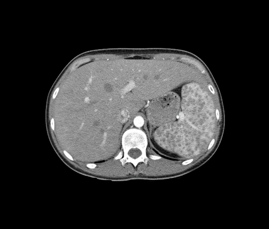
I padded the image on all four sides with a black background to prevent information loss. Since we’re only classifying patches based on the middle pixel, this allows each pixel in the scan to be the middle pixel of one of these patches and to get classified in the training data:
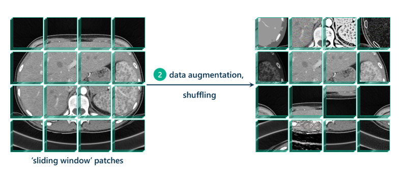
Now that we have our patches, it’s good practice to augment those patches to generate even more data to train the model on. This means replicating patches and tweaking them in different ways, by increasing contrast, lightening, darkening, rotating, cropping, flipping, sharpening, or blurring. Data augmentation allows the model to be more resilient to possible variations in the data that the model will be tested on, which hopefully leads to a more robust, transferable, and adaptable model.
Sampling for data imbalance
There’s one last step before this data can be fed into the model: we need to address the data imbalance. As you might have figured out, there are way more non-lesion patches than there are lesion patches. The ratio turns out to be around 50:1, in fact. Because of this huge class imbalance, the network may have a hard time picking up on the right features that characterize lesion patches. Thus, I needed to under-sample the non-lesion patches to adjust this ratio back to something more reasonable.
As a heuristic, I chose 2:1, since it seemed that 1:1 might run the risk of not properly representing the non-lesion samples, but something higher might again result in class imbalance. I ended up with around 122,000 patches in that 2:1 ratio to train my model with.
Stay tuned for my next post where I return to my deep learning model with fresh eyes.


1 Comment
Pingback: Refining a deep learning model for object detection - The SAS Data Science Blog