This is the second post in my series about a computer vision project I worked on at SAS. In my previous post, I talked about my initial research and excitement for the project. In this post, I’ll talk about how I refined my goals and got started with the project to segment liver tumors in 3D CT scans.

Now that I had a feel for the tools I’d be working with and the end goal of the project, it was time for me to read up on the specific subset of subject matter I’d be tackling:

• What is a dicom image format, and how does it differ from jpeg or png?
• What does the data look like?
• How can I access it, and after that, how do I read it?
• What does a liver look like? What is considered a lesion?
• What is the reasoning behind wanting to extract these lesions from the CT scan?
• How would these resulting segmentations be used?
• How could I make these results most tangible to the user of my end product?

These contextual questions are just as important as understanding the tools I’d be using. They provide motivation for the project, in every sense of the word—a concrete reason the project is important for SAS and for society, as well as intrinsic motivation and excitement for me to want to get it done.

The questions also provided direction for refining the end goal of the project and the steps to get it done. Developing and answering these questions was a crucial checkpoint for the project trajectory and the anticipated final deliverable.

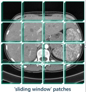
We decided my goal would be to develop a model that used the sliding window approach to segment the lesions from the original raw input images and output a final black-and-white segmentation that could be viewable by the user.

The sliding window approach is a computer vision technique that moves a bounded box around an image looking for the presence of an object in that section of the image each time it moves.

Now that the project was fully defined, I was itching to get going,

Starting with deep learning

Though my final goal was to build a system that took an input and delivered an output, the core component of this system was a deep learning model. My goal was to build a model that would perform the classification task for image segmentation using transfer learning. So that’s where I started.

The first thing I learned about deep learning? Much of it is trial and error. Prior knowledge, educated guesses, empirical evidence, and trying things out are your best friend. You start with a model architecture from the literature, try to replicate that experiment, get a good result, and move on from there.

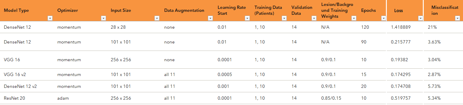
The first thing I learned about #deeplearning? Much of it is trial and error. Prior knowledge, educated guesses, empirical evidence, and trying things out are your best friend. Click To Tweet

As I was using the Python client for Viya, the first thing I did was start several Jupyter notebooks for conducting these experiments. This trial-and-error period ran for about three to four weeks. I explored a few of the various models offered in Viya: DenseNet, VGG, and ResNet. I kept a spreadsheet log of all the hyperparameters (different aspects of the network that can be tweaked, such as learning rate, L2 regularization, and number of epochs run).

As with any complex problem, it was important to start small. In this case, that means I started with smaller models and data to learn what hyperparameters would be optimal for this particular type of data. While CT scans are 3D images with hundreds of slices, here, I started by selecting only a few slices from different patient scans for training the model and then testing on a single slice from a different patient.

At the end of the long process of testing many different combinations of hyperparameters for each of the models, I found that the VGG16 model was the best performer and found the corresponding hyperparameters that maximized its classification efficacy.

At this point, I was about halfway through the project, and I had come up with a rough sketch of the best model that could be used at the core of my pipeline. But there was a lot left to do to turn this single pipe into, well, a line of pipes. Check back soon for my next post where I’ll explain how I did that.

Learn how to do deep learning with SAS