The DO Loop
Statistical programming in SAS with an emphasis on SAS/IML programs
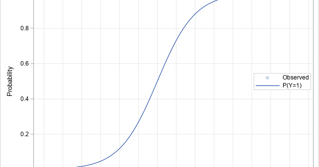
This article shows that you can use the intercept parameter to control the probability of the event in a simulation study that involves a binary logistic regression model. For simplicity, I will simulate data from a logistic regression model that involves only one explanatory variable, but the main idea applies

In a previous article, I presented some of the most popular blog posts from 2022. In general, popular articles deal with elementary topics that have broad appeal. However, I also write articles about advanced topics. The following articles didn't make the Top 10 list, but they deserve a second look.

Since 2008, SAS has supported an interface for calling R from the SAS/IML matrix language. Many years ago, I wrote blog posts that describe how to call R from PROC IML. For SAS 9.4, the process of installing R and calling R from PROC IML is documented in the SAS/IML
