A moving average is a statistical technique that is used to smooth a time series. My colleague, Cindy Wang, wrote an article about the Hull moving average (HMA), which is a time series smoother that is sometimes used as a technical indicator by stock market traders. Cindy showed how to compute the HMA in SAS Visual Analytics by using a GUI "formula builder" to compute new columns in a data table. This article shows how to implement the Hull moving average in the SAS/IML language. The SAS/IML language is an effective way to implement new (or existing) smoothers for time series because it is easy to use lags and rolling windows to extract values from a time series.

I have previously written about how to compute common moving averages in SAS/ETS (PROC EXPAND) and the DATA step. I have also shown how to compute a weighted moving average (WMA) in the SAS/IML language, which includes simple moving averages and exponential moving averages. This article shows how to implement the Hull moving average formula in SAS by leveraging the WMA function in the previous article.

Every choice of weights in a weighted moving average leads to a different smoother. This article uses weights that are linear in time. Specifically, if Y is a time series, the weighted moving average at time index t is obtained by the formula
WMA(t, n) = 1*Y[t − n + 1] + 2*y[t − n + 2] + 3*Y[t − n + 3] + ... + n*Y[t]) / (1 + 2 + ... + n)
In general, the divisor in the formula is the sum of whatever weights are used.

Although this article focuses on the Hull moving average, the techniques are broadly applicable to other moving average computations.

Hull moving average

Cindy's article contains formulas that show how to compute the Hull moving average (HMA). The HMA is the moving average of a linear combination of two other weighted moving averages, one on a shorter time scale and the other on a longer time scale. Given a time series, Y, choose a lag time, n, which is sometimes called the window length. You can compute the Hull moving average by computing four quantities:

1. Compute X_short as the weighted moving average of Y by using a short window of length n/2.
2. Compute X_long as the weighted moving average of Y by using the longer window of length n.
3. Define the series X = 2* X_short – X_long.
4. The Hull moving average of Y is the weighted moving average of X by using a window of length sqrt(n).

The following SAS/IML program implements the Hull moving average. The WMA function is explained in my previous blog post. The HMA function computes the Hull moving average by calling the WMA function three times, twice on Y and once on X. It requires only four statements, one for each computed quantity:

proc iml;
/* Weighted moving average of k data values.
   First k-1 values are assigned the weighted mean of all preceding values.
   Inputs:     y     column vector of length N >= k
               wt    column vector of weights. w[k] is weight for most recent 
                      data; wt[1] is for k time units ago.  The function 
                     internally standardizes the weights so that sum(wt)=1.
   Example calls: 
   WMA  = WMA(y, 1:5);          is weighted moving average of most recent 5 points
   SMA  = WMA(y, {1 1 1 1 1});  is simple moving average of 
   See https://blogs.sas.com/content/iml/2016/02/03/rolling-statistics-sasiml.html
*/
start WMA(y, wt);
   w = colvec(wt) / sum(wt);         /* standardize weights so that sum(w)=1 */
   k = nrow(w);                      /* length of lag */
   MA = j(nrow(y), 1, .);
   /* handle first k values separately */
   do i = 1 to k-1;
      wIdx = k-i+1:k;                /* index for previous i weights */
      MA[i] = sum(wt[wIdx]#y[1:i]) / sum(wt[wIdx]);  /* weighted average */
   end;
   /* main computation: average of current and previous k-1 data values */
   do i = k to nrow(y);
      idx = (i-k+1):i;               /* rolling window of k data points */
      MA[i] = sum( w#y[idx] );       /* weighted sum of k data values */
   end;
   return ( MA );
finish;
 
/* Hull moving average HMA(y, nLag) at each time point. All computations
   use linear weights 1:k for various choices of k. */
start HMA(y, nLag);
   Xshort = WMA(y, 1:round(nLag/2)); /* short smoother (nLag/2) */
   Xlong = WMA(y, 1:nLag);           /* longer smoother (nLag) */
   X = 2*Xshort - Xlong;             /* combination of smoothers */
   HMA = WMA(X, 1:round(sqrt(nLag)));/* Hull moving average (length sqrt(nLag)) */
   return HMA;
finish;
 
/* test on simple time series */
y = T({0 1 0 1 3 2 3 3});
nLag = 4;
WMA = WMA(y, 1:nLag);  
HullMA = HMA( y, nLag );  
print y WMA HullMA;

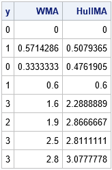
The table shows the weighted moving average and the Hull moving average applied to a simple time series with eight observations. The smoothed values are shown. As a general rule, the Hull moving average tends to be smoother than a raw weighted moving average. For a given lag parameter, it responds more quickly to changes in Y.

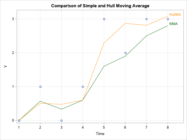
However, it is important to realize that the HMA is not a smoother of Y. Rather, it smooths a linear combination of other smoothers. Consequently, the value of the HMA at time t can be outside of the range of the series {Y₁, Y₁, ..., Y_t}. This is seen in the last observation in the table. The HMA has the value 3.08 even though the range of Y is [0, 3]. This is shown in the following graph, which plots the series, the weighted moving average, and the Hull moving average.

The Hull moving average applied to stock data

This section reproduces the graphs in Cindy's blog post by applying the Hull moving average to the monthly closing price of IBM stock. The following statements compute three different moving averages (Hull, simple, and weighted) and use PROC SGPLOT to overlay the simple and Hull moving averages on a scatter plot that shows the closing price and a high-low plot that shows the range of stock values for each month.

use Sashelp.Stocks where(stock='IBM');       /* read stock data for IBM */
read all var {'Close'} into y; close;
 
nLag = 5;
SMA = WMA(y, j(1,nLag,1));                   /* simple MA */
WMA = WMA(y, nLag);                          /* weighted MA */
HMA = HMA(y, nLag);                          /* Hull MA */
create out var {SMA WMA HMA}; append; close; /* write moving averages to SAS data set */
QUIT;
 
data All;                                    /* merge data and moving averages */
   merge Sashelp.Stocks(where=(stock='IBM')) out;
run;
 
ods graphics / width=800px height=300px;
title "Comparison of Simple and Hull Moving Average";
proc sgplot data=All noautolegend;
   highlow x=Date high=High low=Low / lineattrs=(color=LightGray);
   scatter x=Date y=Close / markerattrs=(color=LightGray);
   series x=Date y=SMA / curvelabel curvelabelattrs=(color=DarkGreen) lineattrs=(color=DarkGreen);
   series x=Date y=HMA / curvelabel curvelabelattrs=(color=DarkOrange) lineattrs=(color=DarkOrange);
   refline '01JUN1992'd / axis=x label='June 1992' labelloc=inside;
   xaxis grid display=(nolabel); 
   yaxis grid max=200 label="IBM Closing Price";
run;

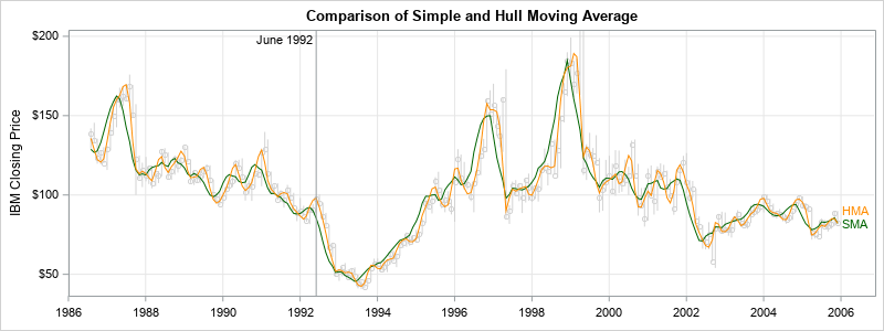
It is well known that the simple moving average (green line) lags the data. As Cindy points out, the Hull moving average (orange line) responds more quickly to changes in the data. She compares the two smoothers in the months after June 1992 to emphasize that the HMA is closer to the data than the simple moving average.

In summary, this article shows how to implement a custom time series smoother in SAS. The example uses the Hull moving average and reproduces the computations and graphs shown in Cindy's article. The techniques apply to any custom time series smoother and time series computation. The SAS/IML language makes it easy to compute rolling-window computations because you can easily access segments of a time series.