SAS graphs for R programmers - maps from shapefiles

This is another in my series of blog posts where I take a deep dive into converting customized R graphs into SAS graphs. Today we'll be working on shapefile maps ...

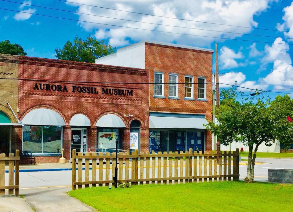
And what data will we be using this time? Here's a hint - the picture below is the Aurora Fossil Museum (near the coast in Aurora, NC). There's a huge phosphate mine beside the town, and fossil hunters who have been fortunate enough to look through the spoil piles have found some really cool fossils over the years. The most popular are probably teeth from megalodon sharks - 50 ft sharks that lived millions of years ago. Some of the megalodons had teeth 6 to 7 inches long (you could win one of these teeth in the museum's raffle, and help them recover from the covid closure, by the way!)

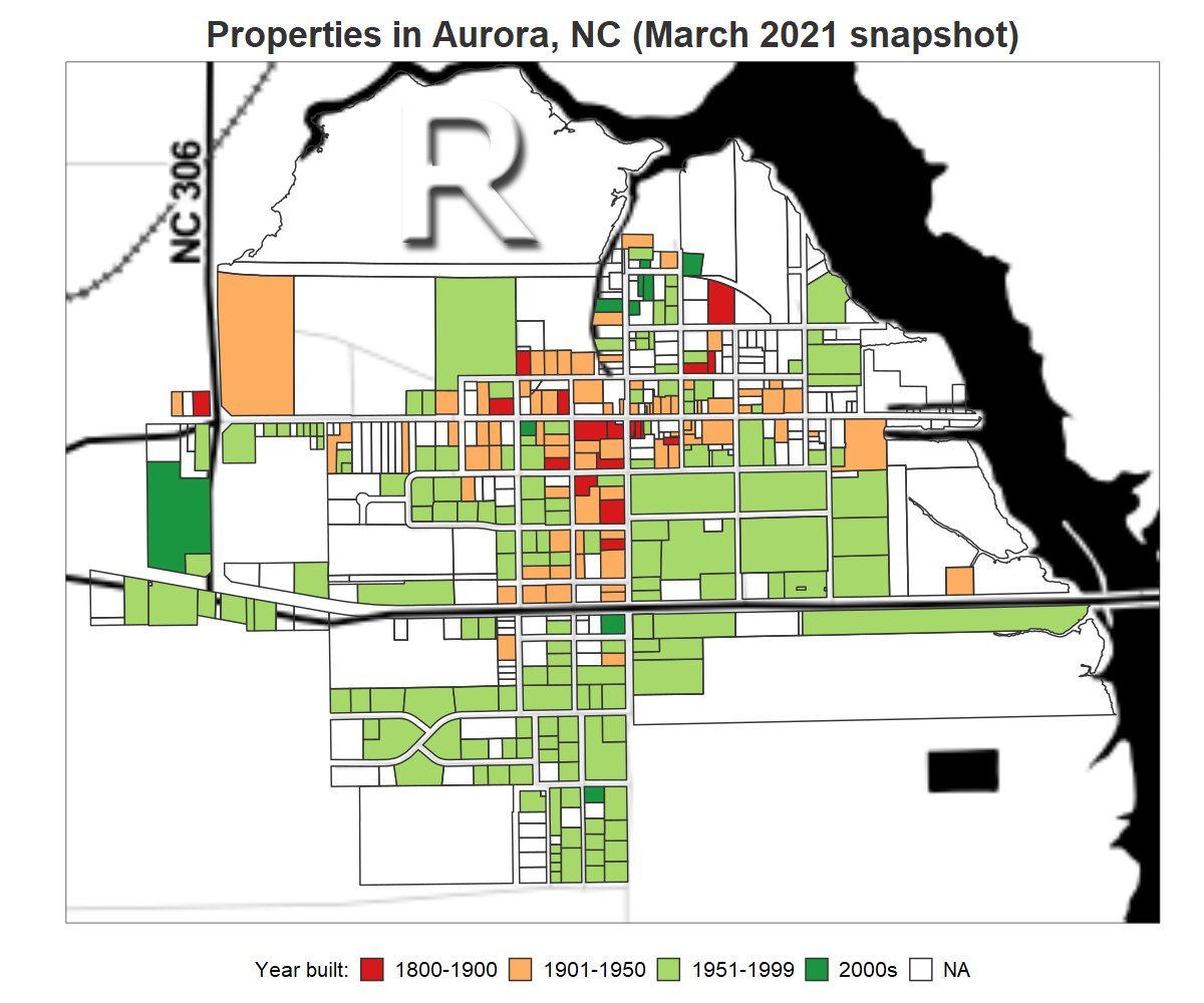
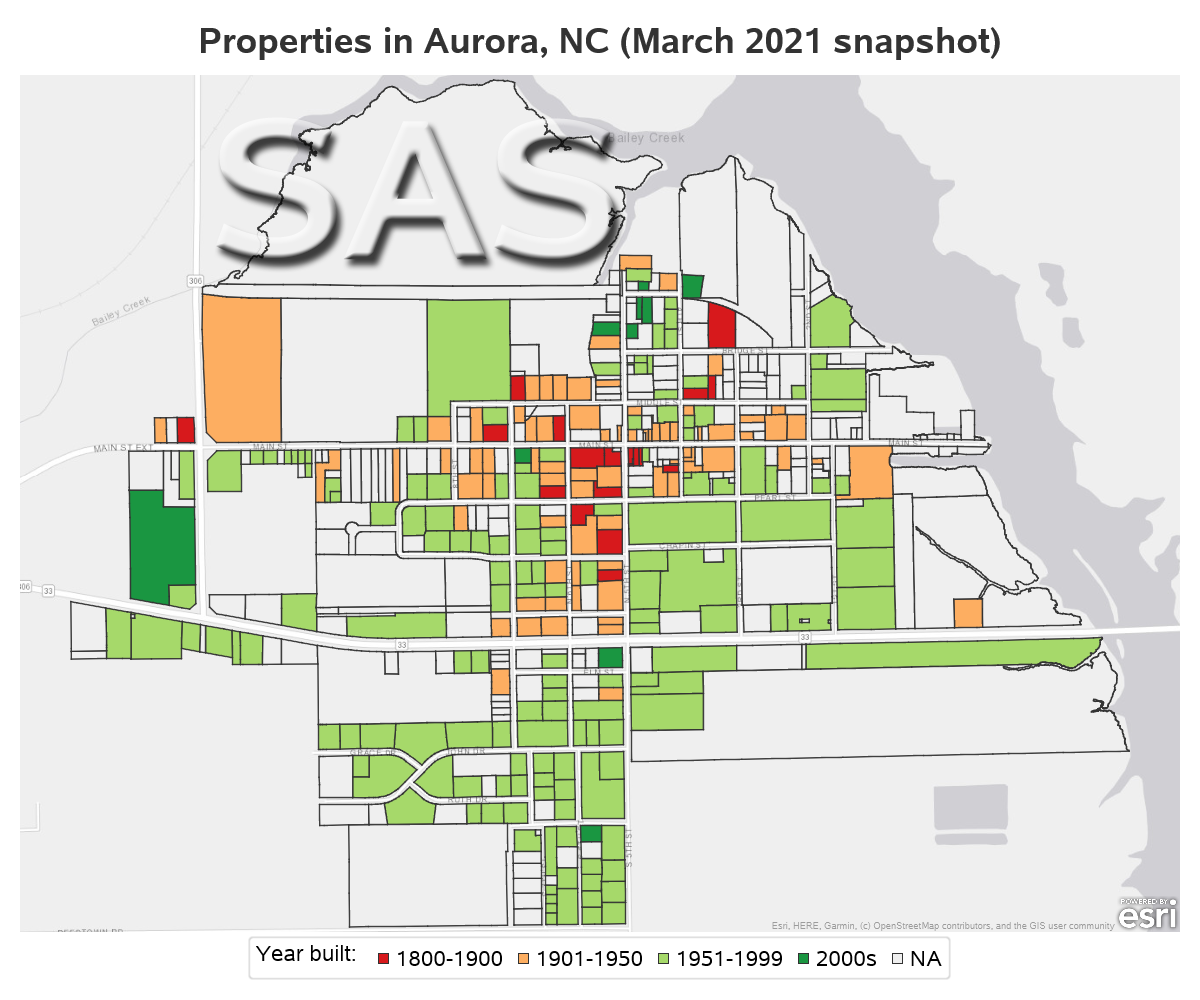
And speaking of old things in Aurora ... I'll be plotting the age of Aurora's houses, on a map of the city! Below are the maps I created using R and SAS:

R Map from Shapefile

SAS Map from Shapefile

My Approach

I will be showing the R code (in blue) first, and then the equivalent SAS code (in red) that I used to create both of the maps. Note that there are many different ways to accomplish the same things in both R and SAS - and the code I show here isn't the only (and probably not even the 'best') way to do things. If you know of a better/simpler way to code it, feel free to share your suggestion in the comments!

Also, I don't include every bit of code here in the blog post (in particular, things I've already covered in my previous posts). I include links to the full R and SAS programs at the bottom.

Getting the Shapefile and Data

Here in North Carolina, property (land & houses) is generally kept track of at the county level. There are 100 counties in NC, and each county has several cities. A piece of land is generally referred to as a parcel, and many counties provide geographical descriptions of the borders of the parcels in the form of shapefiles.

Aurora, NC is located in Beaufort county (pronounced bow-fort ... not to be confused with Beaufort, SC which is pronounced beau-fert), and they provide a shapefile for their entire county on their webpage. Here's what the link looks like:

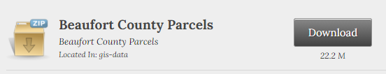
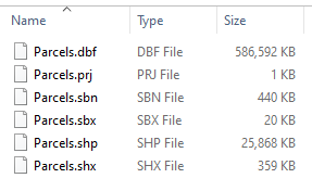
I downloaded and extracted the zip, and ended up with the following files:

Importing the Shapefile

In R, I used the readOGR() function to import the county shapefile, and store it as a spatial points data frame (spdf). Note that it took several minutes for readOGR() to run. I then limited it to just the parcels within the city limit of Aurora (aka, Township 13). And finally use the spTransform() function, to convert the X and Y values into the longitude and latitude values in degrees that we typically work with. And finally the tidy() function converts the spdf into a regular R data frame containing polygons that can be plotted by the geom_polygon() function.

county_spdf <- readOGR(dsn="D:/Public/beaufort_county/Parcels.shp",verbose=FALSE)

city_spdf <- subset(county_spdf,TOWNSHIP=='13')

city_spdf <- spTransform(city_spdf,"+init=epsg:4326")

city_frame <- tidy(city_spdf,region="GPINLONG")

In SAS I use Proc Mapimport to import the shapefile. This ran in 23 seconds on my laptop (by comparison, it took R several minutes to import the shapefile). Note that although we only specify the .shp file, the proc assumes the other files are there in the same folder. I then use a data step to limit it to just the parcels within the city limit of Aurora (Township 13). And finally use Proc Gproject (now included with Base SAS) to convert the X and Y values into the longitude and latitude values in degrees (note that I had to specify both the from= and to= coordinate system here, whereas in R I only had to specify the coordinate system I was converting to). You have to do some digging to figure out what the from= coordinate system should be.

proc mapimport datafile="D:\Public\beaufort_county\Parcels.shp" out=county_map;
run;

data city_map; set county_map (where=(township='13'));
run;

proc gproject data=city_map out=city_map from="EPSG:2264" to="EPSG:4326";
id;
run;

Response Data

There's a lot of information about each parcel in the shapefile, such as value, acres, owner, year built, etc. I plan to use the year built to color the polygons, and several of the variables to provide information in the mouse-over text. But the R function that converts the spdf into a data frame gets rid of all the extra information (it only keeps the bare bones info it needs for the polygon geometry). Therefore I had to extract that extra information from the spdf, assign mnemonic variable names using the names() function, and then use the join() function to merge it back into the polygon frame data. Note that I change the name of the GPINLONG (parcel identification number) variable to 'id', so that I can use it in the join.

temp_unique <- data.frame(
city_spdf@data$GPINLONG,
city_spdf@data$PROP_ADDR,
city_spdf@data$CalcAcres,
city_spdf@data$TOT_VAL,
city_spdf@data$YR_BUILT,
city_spdf@data$NAME1,
city_spdf@data$NAME2)
names(temp_unique) <- c("id","PROP_ADDR","CalcAcres","TOT_VAL","YR_BUILT","NAME1","NAME2")
city_frame_plus <- join(city_frame,temp_unique,by="id")

Next I use R's ifelse statements to assign values to a special yr_built_range variable. And in the final step I use the paste() function to create a long text variable containing all the information I want in the mouse-over text (notice I use ' ' to insert line breaks between the values).

city_frame_plus <- city_frame_plus %>% mutate(
city_frame_plus, yr_built_range=
ifelse(YR_BUILT<=1900,'1800-1900',
ifelse(YR_BUILT<=1950,'1901-1950',
ifelse(YR_BUILT<=1999,'1951-1999',
ifelse(YR_BUILT>=2000,'2000s',
'NA')))))

city_frame_plus$tooltip_text <- paste(
"ID: ",city_frame_plus$id," ",
"Address: ",city_frame_plus$PROP_ADDR," ",
"Acres: ",city_frame_plus$CalcAcres," ",
"Value: ",format_dollars(city_frame_plus$TOT_VAL)," ",
"Year built: ",city_frame_plus$YR_BUILT," ",
"Owner: ",city_frame_plus$NAME1," ",
"Owner 2: ",city_frame_plus$NAME2,
sep=" ")

In R I used a general polygon plotting function to draw the polygons, and both the polygon and the response data needed to be in the same dataset (see the 'join' above) ... whereas in SAS we'll be using a specialty map-drawing procedure, and the map polygons and response data need to be in separate datasets. Proc Mapimport stores both the polygon and response data together, therefore in SAS we need to separate out the response data. I do this with Proc SQL.

proc sql noprint;
create table my_mapdata as
select unique gpinlong, tot_val, calcacres, name1, name2, prop_addr, township,
condition, road_type, roof_mater, sq_ft, use_desc, utility, wall, yr_built,
from city_map;
quit; run;

I then assign labels to the variables, so they'll have nice descriptions in the mouse-over text:

data my_mapdata; set my_mapdata;
label gpinlong='Parcel ID';
label tot_val='Value';
label prop_addr='Address';
label use_desc='Use';
label wall='Wall material';
label yr_built='Year built';
label roof_mater='Roof material';
format sq_ft_num comma8.0;
sq_ft_num=.; sq_ft_num=sq_ft;
label sq_ft_num='Square ft';
label condition='Condition';
label calcacres='Acres';
label road_type='Road type';
label utility='Utilities';
label name1='Owner';
label name2='Owner 2';
label township='Township';
format tot_val dollar10.0;
run;

And finally, I use a SAS data step with if / else statements to assign values to the yr_built_range variable.

data my_mapdata; set my_mapdata;
label yr_built_range='Year built:';
length yr_built_range $20;
if yr_built=. then yr_built_range='NA';
else if yr_built<=1900 then yr_built_range='1800-1900';
else if yr_built<=1950 then yr_built_range='1901-1950';
else if yr_built<=1999 then yr_built_range='1951-1999';
else if yr_built>=2000 then yr_built_range='2000s';
else yr_built_range='NA';
run;

Plotting the Map

To get the desired map, I draw the parcel polygons (choropleth map), shade them based on the year the houses were built (yr_built_range), and overlay those polygons on a background tile-based map of the city.

In R, I first have to get the background tile map. You're probably familiar with the tile-based OpenStreetmaps - that is similar to what I'm using, but I wanted something a little simpler than the typical street maps, with no color (because colors in the background map would compete with the colored parcel polygons I'll be overlaying on the map). In R, I use the get_stamenmap() function to get a black-n-white background map, specifying the exact latitude/longitude extents of the desired map area, and the desired zoom level (this took quite a bit of time using trial-and-error). This map shows the major streets, and bodies of water (Aurora is right on the river/sound).

my_map <- get_stamenmap(bb=c(left=-76.803,bottom=35.294,right=-76.775,top=35.312),zoom=14,maptype="toner")

I then used R's ggmap() to draw the background tile map, and geom_polygon() to draw and color the parcel polygons. Note that geom_polygon() would typically also include graph axes, but I used the theme() to suppress them.

my_plot <-
ggmap(my_map)+
geom_polygon(data=city_frame_plus,color="#333333",
aes(x=long,y=lat,group=group,fill=yr_built_range,text=tooltip_text)) +
scale_fill_manual(name="Year built:",values=c("#d7191c", "#fdae61", "#a6d96a", "#1a9641", "#efefef")) +
xlab('') + ylab('') +
theme_bw() +
theme(axis.line = element_blank(),
axis.text = element_blank(),
axis.ticks = element_blank()
) +
labs(title="Properties in Aurora, NC (March 2021 snapshot)") +
theme(plot.title=element_text(size=26,color="#333333",face="bold",hjust=0.5,margin=margin(10,0,5,0))) +
theme(legend.margin=margin(-2,0,0,0)) +
theme(legend.position="bottom",legend.box.margin=margin(0,0,10,0)) +
theme(legend.title=element_text(size=15)) +
theme(legend.text=element_text(size=15))

In SAS, I used Proc SGmap to draw and color the parcel polygons (choropleth map), and SGmap's esrimap statement to include a black-and-white Esri tile map behind the polygons. Since SGmap is specifically made for drawing maps, there are no axes to get rid of. Also, SGmap automatically determines the background map tiles and zoom level needed, based on the polygon latitude/longitude extents (no need to specify latitude/longitude extents like we did in R - this saved me a lot of time in SAS).

proc sgmap mapdata=city_map maprespdata=my_mapdata;
esrimap url="http://services.arcgisonline.com/arcgis/rest/services/Canvas/World_Light_Gray_Base";
styleattrs datacolors=(cxd7191c cxfdae61 cxa6d96a cx1a9641 cxefefef);
choromap yr_built_range / mapid=gpinlong lineattrs=(color=cx333333);
keylegend / titleattrs=(size=14) valueattrs=(size=14);
run;

Adding Mouse-Over Text

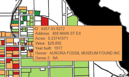
The static image of the map is interesting, but these days people expect a little more interactive behavior in their maps. Therefore I decided to add mouse-over text to the map.

In the previous R code, I had set up the text in the tooltip_text variable, and identified that variable using aes(text=tooltip_text). I used ggsave() to write the map out to a png file, but a png file doesn't have any interactivity such as mouse-over text. Therefore I also used save_html() to write out a second 'interactive html' version of the map, telling it to use the text= I had set up in the aes() as my tooltip mouse-over text. Here's the code, and a screen capture showing what the text looks like. Note that R writes a bunch of stuff to the 'libdir' that is needed to support the mouse-over text.

my_plot1 <- plotly::ggplotly(my_plot,width=1200,height=1000,tooltip="text") %>% layout(autosize=FALSE)
my_plot2 <- htmltools::div(my_plot1,align="center")
htmltools::save_html(my_plot2,paste(name,".htm",sep=""),background="white",libdir="shared_lib")

It's a little easier to get the mouse-over text in SAS. I use Proc SGmap's tip= option to list the variables I want to show in the mouse-over text. SAS 'ODS Html' writes out a png image of the map, and an HTML file that points to the png, and defines areas for the polygons, and uses HTML alt= and title= tags to set up the mouse-over text. Just two files, and simple HTML tags.

proc sgmap mapdata=city_map maprespdata=my_mapdata /*noautolegend*/;
esrimap url="http://services.arcgisonline.com/arcgis/rest/services/Canvas/World_Light_Gray_Base";
styleattrs datacolors=(cxd7191c cxfdae61 cxa6d96a cx1a9641 cxefefef);
choromap yr_built_range / mapid=gpinlong lineattrs=(color=cx333333)
tip=(gpinlong prop_addr tot_val yr_built use_desc wall roof_mater sq_ft_num calcacres name1 name2)
keylegend / titleattrs=(size=14) valueattrs=(size=14);
run;

Bonus - Drilldown!

In addition to mouse-over text, users also tend to expect (or at least desire) drilldown capability in maps like this. I experimented a bit with R and couldn't figure out a way to associate drilldown URLs with the parcel polygons there (perhaps you know of a way, and can let me know in a comment).

In SAS, I can set up a variable in the response data that contains the desired URL (which can be generated in a data-driven way, based on the data), and then specify that URL in SGmap's url= option. I don't really have any data pages to drilldown to (such as the property titles, or tax statement), therefore I set up links for the single-family homes to do a Zillow query for that street address, and all other parcels to do a Google map on the latitude/longitude coordinate. Here's a link where you can try out my interactive SAS map with drill-downs.

length lookup_link $300;
if use_desc in ('SINGLE FAMILY RESIDENCE' 'MOBILE HOME' 'MODULAR HOMES') then
lookup_link='https://www.zillow.com/homes/for_sale/'||translate(lowcase(trim(left(prop_addr))),'-',' ')||',-aurora,-nc_rb/';
else
lookup_link='https://www.google.com/maps/@'||trim(left(lat_center))||','||trim(left(long_center))||',20z';
landcolor="foo";

proc sgmap mapdata=city_map maprespdata=my_mapdata;
esrimap url="http://services.arcgisonline.com/arcgis/rest/services/Canvas/World_Light_Gray_Base";
styleattrs datacolors=(cxd7191c cxfdae61 cxa6d96a cx1a9641 cxefefef);
choromap yr_built_range / mapid=gpinlong lineattrs=(color=cx333333)
url=lookup_link;
keylegend / titleattrs=(size=14) valueattrs=(size=14);
run;

More Bonus - More Backgrounds

In R, I could also have used a Google background map, but I would need to sign up for a Google API key, and the Google "terms of service" for that were a little scary (for example, if I followed their terms of service to-the-letter, I don't think I would have been allowed to create this map with a Google tile background and include it in this blog). So I chose to not even try to create an R version.

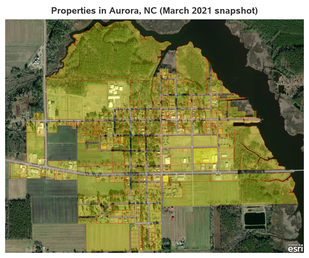
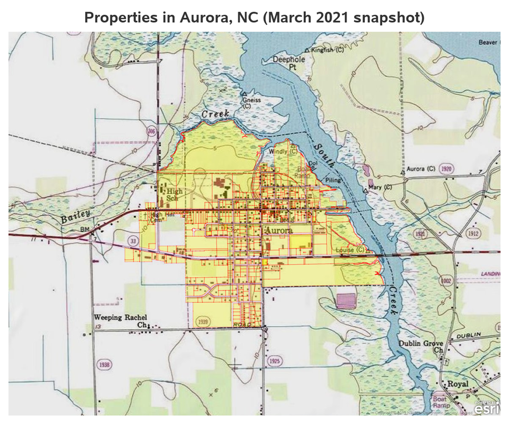
In SAS, you're allowed to choose from a large selection of background maps (from both OpenStreetmaps and Esri). Here are two examples I think are interesting to plot the Aurora parcels on. I just plot the parcel borders (in red), with no fill color here, so you can see the background maps more clearly.

esrimap url="http://services.arcgisonline.com/arcgis/rest/services/World_Imagery";

esrimap url="http://services.arcgisonline.com/arcgis/rest/services/USA_Topo_Maps";

My Code

Here is a link to my complete R program that produced the R map.

Here is a link to my complete SAS program that produced the SAS maps.

If you have any comments, suggestions, corrections, or observations - I'd be happy to hear them in the comments section!

Blogs