Supervised classification does not usually end with an estimate of the posterior probability. For example, in binary classification problems, the ultimate use of a predictive model is to allocate cases to classes by appropriately choosing a posterior probability cutoff. The cutoff or threshold represents the probability that the prediction is true.
Determining an appropriate cutoff is problem-specific and there are many ways of accomplishing this. A formal approach to determining the optimal cutoff uses statistical decision theory. The decision-theoretic approach starts by assigning profit margins to true positives and loss margins to false positives. The optimal decision rule maximizes the total expected profit.
Let’s consider an example of a fictitious telecommunications company seeking to determine which customers might be likely to churn based on demographics, customer care and prior usage of services. The target variable is binary: churner or non-churner. Profit in churn modeling can be evaluated in several ways. One of the most common ways is to consider a matrix that signifies the change in profit by using a churn model over not using it, that is, no intervention model.
A base scenario represents the system without using the recommended model. The baseline is that there is no prediction system and churner customers are not detected by the company and they leave. Consequently, the company loses all the potential profit which could be earned from those customers. Accordingly, all the profits and costs in this study have been calculated based on a base scenario which assumes that there is no churn prediction system.
The ultimate objective of a churn model is preventing churn by making a retention offer. To determine reasonable values for profit and loss information, consider the outcomes and the actions that you would take given knowledge of these outcomes. For example, the marketing department of a telecommunications company wants to offer a discount to people who are no longer on a fixed-term contract. To prevent churn, the company is willing to make an offer in exchange for a one-year contract extension.
In this case, there are two outcomes (churn and no churn) and two corresponding actions (offer discount and no action). Knowing that someone is a churner, you would naturally want to offer a discount to that person. Knowing that someone is a non-churner, you would naturally want to not offer any discount to that person. On the other hand, knowledge of an individual’s actual behavior is rarely perfect, so mistakes are made (for example, offering discounts to non-churners (false positives) and not taking any action for churners (false negatives)). Usually, incorrectly predicted observations have different importance. In this case, false negatives can cost more than false positives.
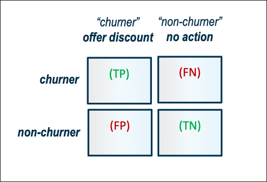
Taken together, there are four outcome-and-action combinations shown in Figure 1. Each of these outcome-and-action combinations has a profit consequence (where a loss is called, somewhat euphemistically, a negative profit).
Suppose from the description of the analysis problem that the variable AVG_ARPU_3M gives average revenue for the past three months (when a customer stays). The average revenue per unit (ARPU) for the past three months means we take the 3-month average of the ARPU (which is itself a monthly average) for that customer. This 3-months is the rolling average window; any dollar value you see would represent a monthly value.
Note: The 'unit' in ARPU could be a landline, cell phone, TV, internet, etc. Each of those units has much different profit margins, by the way. To put it another way, we take the monthly revenue for each of a customer's products and we divide that by the total number of products to arrive at a customer's ARPU. We then take the two previous measurements of ARPU and average them together with the current month to arrive at the AVG_ARPU_3M.
Profit is proportional to the average revenue for the past three months. From a statistical perspective, AVG_ARPU_3M is a random variable. Individuals who are identical on every input measurement might have different average revenue amounts. To simplify the analysis, a summary statistic for AVG_ARPU_3M is plugged into the profit consequence matrix. In general, this value can vary on a case-by-case basis. However, for triviality, the overall average of AVG_ARPU_3M is used (Mean of AVG_ARPU_3M = 60.30$).
Note: Average revenue is commonly considered by average tenure or by customer lifetime value. Although variables ACCT_AGE, that is, account tenure and LIFETIME_VALUE, a customer’s lifetime value might be given in the data, they are not considered here for continuing triviality. Moreover, the profit matrix considered here is on the individual customer level. A simple alternative of considering a time period is how many months you get from saving a churner will suffice. To prevent churn, the company is willing to make a promotion offer in exchange for a one-year contract extension. So, here we can use the 12-month additional profit.
Also, you find that it costs approximately a 15% decline in the average revenue of that customer when a discount is offered to retain that customer (15% of 60.30$ = 9.04$). The company decides to offer the same/fixed retention promotion to all the targeted customers. It is believed that this promotional offer is effective enough to retain the customer.

Churners caught at the beginning of the journey considering the average tenure will represent great revenue savings. This is when you give a 15% discount to customers that you predicted as churn, and in response, they no longer churn. You earn average revenue minus the 15% discount. In other words, $60.30 – $9.04 = $51.26 is the monthly average profit (see Figure 2). These profits and costs are not counted in the base scenario.
As you know, there are several factors that play into why someone churns. Most analytical organizations who are going to employ this method will know an estimate of the effectiveness of the offer. Let's say the effectiveness rate is 60%. This would reduce the monthly profit from $51.26 down to $30.76.
For easiness, let's assume that all churn is based on price and thus the offer is 100% effective.
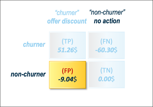
False positive represents the company’s good relationship with the customer. This is when you predict that they churn but they anyway stay. You did give the discount to them, so you lose the profits of the discount. The amount lost is $9.04 (see Figure 3). This represents a substantial missed revenue for the average tenure or for the considered time period.
When you consider the effectiveness rate of taking the offer, you would not reduce your losses because you need to assume that everyone who was planning on staying and is offered a discount will take it. Therefore, unlike TPs, this value would not go down.

This is when the model predicts customers stay while customers actually churn. Although we lose that customer’s potential profit, we cannot consider it as a cost because in the base scenario, this customer’s profit was lost as well and we have no added cost compared with the base scenario (see Figure 4).
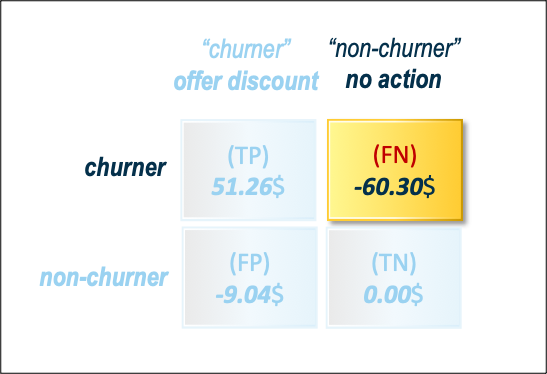
However, false negatives are the costliest classification error in typical churn modeling. When the model predicts customers stay, there is no need to give discount incentives for these customers. The company thereby loses profits by making them leave without doing any action for them to stay. Whereas, in terms of false positives (the model predicts customers churn while they stay), the company reduces profits by offering discounts, but still has some revenue from these returning customers. It is important, therefore, to minimize our false negative rate (or minimize costs) while maximizing the true positive rate (maximize profits).
Here potential loss of $60.30 is considered and this would make the best model the one that minimizes the FNs (see Figure 5).
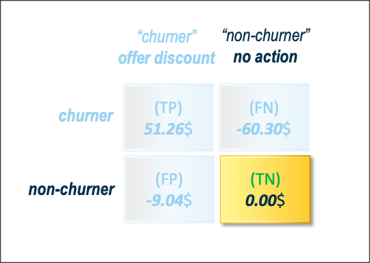
This is when you predict customers do not churn, so you do not give discounts to them and they actually stay. You earn profits as usual. If the customer does not churn, it has no effect on your model. So, the value can immediately be set to 0 (see Figure 6).
The individual customer monthly net profit matrix for churn prediction is given as follows:
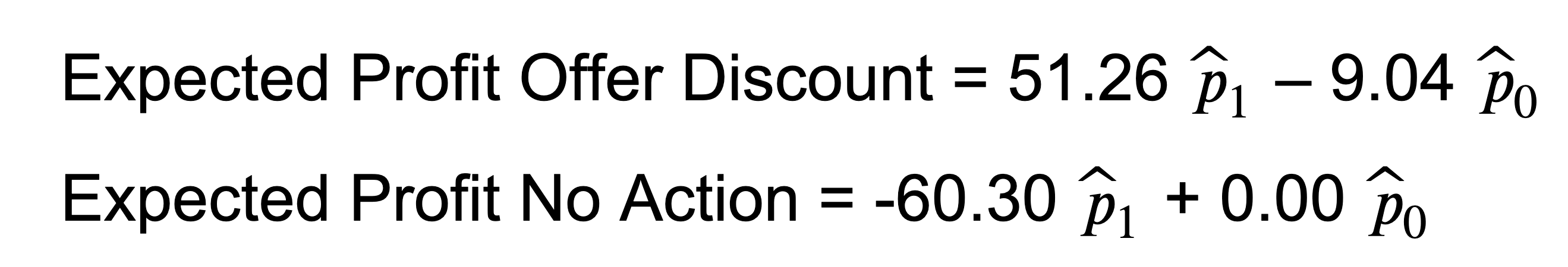
With the completed profit consequence matrix, you can calculate the expected profit associated with each decision. This is equal to the sum of the outcome and action profits multiplied by the outcome probabilities. The best decision for a case is the one that maximizes the expected profit for that case.
Note: We often focus predictive analytics on modeling customer churn. On the other hand, incremental response modeling (also called net lift modeling) takes a different approach. This technique is often used to identify the customers most likely to act upon receiving a “retention offer,” such as a promotional email. The objective of incremental response modeling is to answer this question: Which customers stay only if they are offered a retention promotion by a marketing action? However, in this analysis, it is assumed that the churn probability of a customer before and after making a promotion offer remains the same.
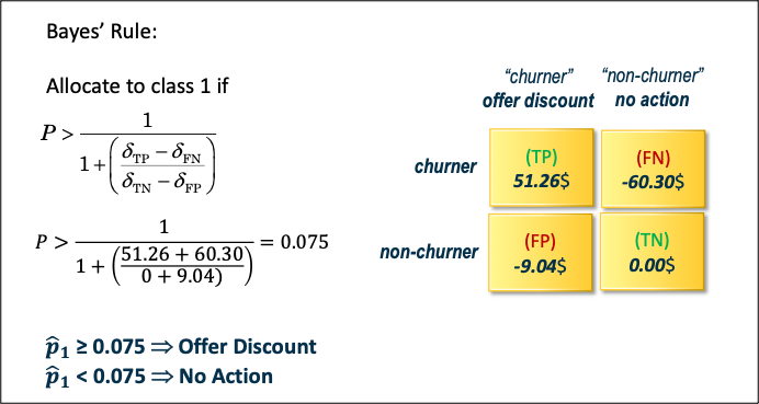
When the elements of the profit consequence matrix are constants, prediction decisions depend solely on the estimated probability of response and a constant decision threshold, as shown in Figure 7.
The HPDECIDE procedure creates optimal decisions that are based on a decision matrix that you specify, on prior probabilities, and on output from a modeling procedure (see Figure 8). This output can be either posterior probabilities for a categorical target variable or predicted values for an interval target variable. The HPDECIDE procedure can also adjust the posterior probabilities for changes in the prior probabilities.
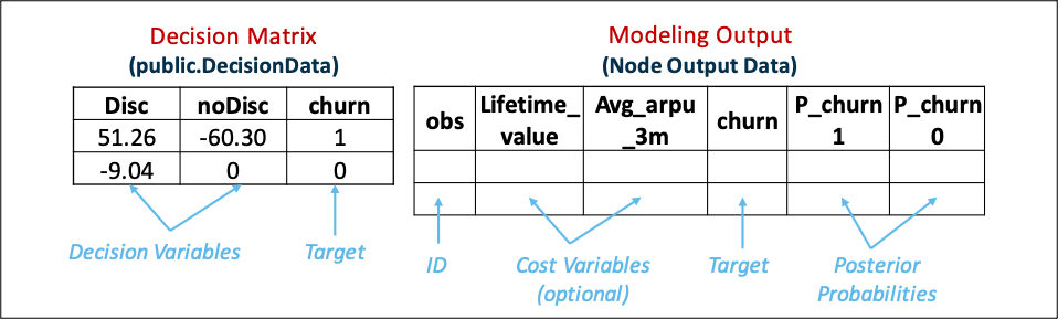
Each modeling node can make a decision for each case in a scoring data set, based on numerical consequences specified via a decision matrix and cost variables or cost constants. The decision matrix can specify profit, loss, or revenue. With a previously scored data set containing posterior probabilities, decisions can also be made using PROC HPDECIDE, which reads the decision matrix from a decision data set.
The decision matrix contains columns (decision variables) that correspond to each decision and rows (observations) that correspond to target values. The values of the decision variables represent target-specific consequences, which might be profit, loss, or revenue. These consequences are the same for all cases that are scored.
For each decision, there might also be either a cost variable or a numeric constant. The values of these variables represent case-specific consequences, which are always costs. These consequences do not depend on the target values of the cases that are scored. Costs are used for computing return on investment as (revenue – cost) / cost.
Cost variables might be specified only if the decision data set contains revenue, not profit or loss. Therefore, if revenues and costs are specified, profits are computed as revenue minus cost. If revenues are specified without costs, the costs are assumed to be 0. The interpretation of consequences as profits, losses, revenues, and costs is needed only to compute return on investment. You can specify values in the decision data set that are target-specific consequences, but that might have some practical interpretation other than profit, loss, or revenue. Likewise, you can specify values for the cost variables that are case-specific consequences, but that might have some practical interpretation other than costs. If the revenue/cost interpretation is not applicable, the values that are computed for return on investment might not be meaningful.
The HPDECIDE procedure chooses the optimal decision for each observation. If the type of decision data set (as specified in the DECISION statement) is PROFIT or REVENUE, PROC HPDECIDE chooses the decision that produces the maximum expected or estimated profit. If the type is LOSS, PROC HPDECIDE chooses the decision that produces the minimum expected or estimated loss.
Model profit is calculated using a profit matrix in the HPDECIDE procedure in a SAS Code node in Model Studio. A vast simplification and common practice in the prediction is to assume that the profit associated with each case, outcome and decision is a constant. This is the default behavior of the HPDECIDE procedure.
A SAS code node is connected to the Logistic Regression node. Several models were created, however, the profit approach is shown on the logistic regression as an illustration.

Following program is used the Code Editor window of the SAS Code node. First, a CAS session was started and all the default libraries were assigned.
options cashost='&dm_cashost' casport=&dm_casport; cas; caslib _all_ assign; |
Next, part of the program loads the decisionData.csv file from a client location into the specified caslib and saves it with specified table name.
proc CASUTIL; load file="/workshop/ADML/decisionData.csv" importoptions=(filetype="csv") outcaslib= "public" casout="decisionData"; *promote; run; |
The following piece of code creates optimal decisions that are based on a decision matrix that you specify, on prior probabilities and on output from a modeling node. This output can be either posterior probabilities for a categorical target variable or predicted values for an interval target variable.
proc HPDECIDE data=&dm_data out=outBayes outstat=outstatBayes; decision decdata=public.DecisionData (type=profit) decvars=Disc noDisc; posteriors p_churn1 p_churn0; target %dm_dec_target; performance details nthreads=2; run; |
The PROC HPDECIDE statement invokes the procedure and identifies the input and output data sets.
The DECDATA= option in the DECISION statement names the input data set that contains the decision matrix or the prior probabilities, or both. This argument is required. The data set option TYPE= is specified in parentheses after the data set name when the data set is created or used. The possible values of TYPE= are LOSS, PROFIT, and REVENUE. The default is PROFIT.
The POSTERIORS statement specifies a list of the numeric variables in the input data set that contain the estimated posterior probabilities that correspond to the categories of the target variable.
The TARGET statement specifies which variable is the target variable in the data set that is specified in the DECDATA= option in the DECISION statement. The TARGET statement is required.
The estimated posterior probabilities that correspond to the categories of the target variable churn are denoted by p_churn1 and p_churn0. You can include two cost variables that represent the target-specific consequences for the decision variables Disc and noDisc, respectively. No cost variables are used in this example.
The last piece of code prints the first 20 observations of the desired output. Also, the profit table is printed.
proc PRINT data=outBayes (obs=20); var p_churn1 p_churn0 I_churn F_churn Disc noDisc D_decisionData EP_decisionData CP_decisionData; run; proc PRINT data=outstatBayes; run; |
After running the SAS Code node, the following results were obtained:
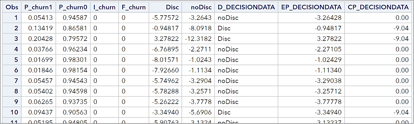
The table shows the outBayes data set, which displays the decision for each observation.
- I_churn specifies the normalized category that the case is classified into.
- F_churn specifies the normalized category that the case comes from.
- D_DecisionData is the label of the decision chosen by the model.
- EP_ DecisionData is the expected profit for the decision chosen by the model.
- CP_ DecisionData is the profit computed from the target value. The value 0 signifies no change in the usual profit.
For example, the predicted probability of churn for the first observation is 0.0541. Expected change in profits for decisions that offer a discount, and no action are $-5.7757 and $-3.2643, respectively. Because the latter is larger, the decision is to not offer a discount, reflected in the D_ column, and the expected profit for this observation would be $-3.2643, reflected in the EP_ column. This is underscored by the fact of the optimal Bayes’ decision threshold. This says to offer the discount if the predicted probability of churn is greater than or equal to 0.0756.
The profit table is also printed:

Average profit can be used to summarize model performance. For the profit matrix used, average profit is computed by multiplying the number of cases by the corresponding profit in each outcome-and-decision combination, adding across all outcome-and-decision combinations, and dividing by the total number of cases in the assessment data.
The outstatBayes data set shows that the total (monthly) profit is $24,625.28 and the average profit is $0.43541, based on the decisions from the outBayes data set. If you would like to compute the total profit for a one-year contract extension, multiply $24,625.28 by 12 months.