When shopping for a new TV, with many sets next to each other across a store wall, it is easy to compare the picture quality and brightness. What is not immediately evident and expected is the difference between how the set looked in the store and how it looks in your home. HDTV pictures are calibrated by default for large bright stores, as that is where the purchase decision is made. In most cases, the backlight setting for LED HDTVs is set at the factory at its maximum setting for bright display in stores. Many other adjustable settings also affect the quality of the picture – brightness, contrast, sharpness, color, tint, color temperature, picture mode, and other more advanced picture control options like motion mode and noise reduction. While most people simply connect the TV and use out-of-the-box settings, not having been instructed in the past to adjust the TV, it turns out that modern HDTVs need to be calibrated to the room size and typical lighting, which will vary. Simply reducing the backlight can make a huge difference (in my case, I reduced this setting from the peak of 20 down to 6!). Adjusting all the options manually, independently, can be tricky. Luckily there are online recommendations for most TV models for the average room. This can be a good start, but again, each room will be different. Calibration discs and/or professional calibration technicians can help to truly find an optimal setting for your environment, to tweak advanced settings. Wouldn’t it be nice if a TV could calibrate itself to its environment? Perhaps this is not far off, but for now the calibration is a manual process.

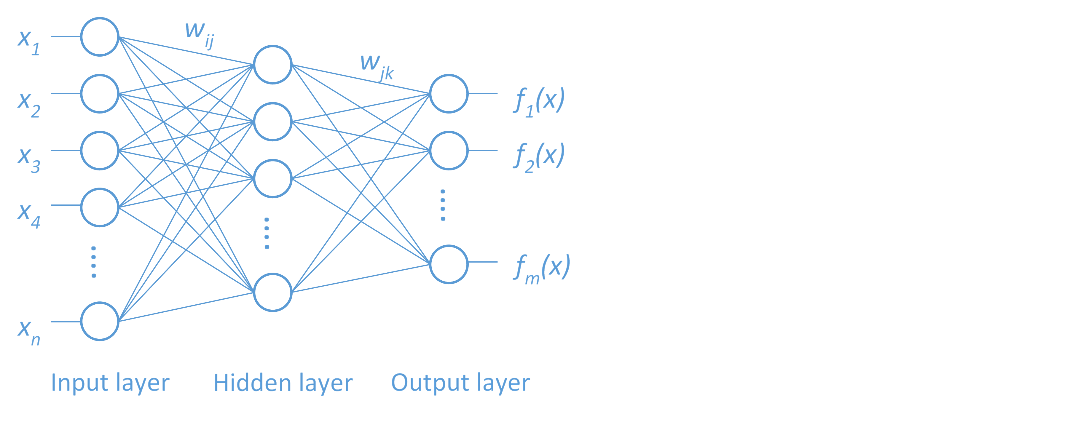
Once a TV is calibrated, it is ready to enjoy. The visual data, the broadcasted information, can be observed, processed, and understood in real time. When it comes to data analytics, however, with raw data in the form of numbers, text, images, etc., gathered from sensors and online transactions, ‘seeing’ the information contained within, as the source grows rapidly, is not so easy. Machine learning is a form of self-calibration of predictive models given training data. These modeling algorithms are commonly used to find hidden value in big data. Facilitating effective decision making requires the transformation of relevant data to high-quality descriptive and predictive models. The transformation presents several challenges however. As an example, take a neural network (Figure 1). A set of outputs are predicted by transforming a set of inputs through a series of hidden layers defined by activation functions linked with weights. How do we determine the activation functions and the weights to determine the best model configuration? This is a complex optimization problem.

The goal in this model training optimization problem is to find the weights that will minimize the error in model predictions given the training data, validation data, specified model configuration (number of hidden layers, number of neurons in each hidden layer) and regularization levels designed to reduce overfitting to training data. One recently popular approach to solving for the weights in this optimization problem is through use of a stochastic gradient descent (SGD) algorithm. The performance of this algorithm, as with all optimization algorithms, depends on a number of control parameters for which no set of default values are best for all problems. SGD parameters include among others a learning rate controlling the step size for selecting new weights, a momentum parameter to avoid slow oscillations, a mini-batch size for sampling a subset of observations in a distributed environment, and adaptive decay rate and annealing rate to adjust the learning rate for each weight and time. See related blog post ‘Optimization for machine learning and monster trucks’ for more on the benefits and challenges of SGD for machine learning.

The best values of the control parameters must be chosen very carefully. For example, the momentum parameter dictates whether the algorithm tends to oscillate slowly in ravines where solutions lie, jumping across the ravine, or dives in quickly. But if momentum is too high, it could jump by the solution (Figure 2). The best values for these parameters also vary for different data sets, just like the ideal adjustments for an HDTV depending the characteristics of its environment. These options that must be chosen before model training begins dictate not only the performance of the training process, but more importantly, the quality of the resulting model – again like the tuning parameters of a modern HDTV controlling the picture quality. As these parameters are external to the training process – not the model parameters (weights in the neural network) being optimized during training – they are often called ‘hyperparameters’. Settings for these hyperparameters can significantly influence the resulting accuracy of the predictive models, and there are no clear defaults that work well for different data sets.

In addition to the optimization options already discussed for the SGD algorithm, the machine learning algorithms themselves have many hyperparameters. Following the neural net example, the number of hidden layers, the number of neurons in each hidden layer, the distribution used for the initial weights, etc., are all hyperparameters specified up front for model training that govern the quality of the resulting model.

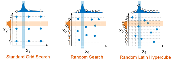
The approach to finding the ideal values for hyperparameters, to tuning a model to a given data set, traditionally has been a manual effort. However, even with expertise in machine learning algorithms and their parameters, the best settings of these parameters will change with different data; it is difficult to predict based on previous experience. To explore alternative configurations typically a grid search or parameter sweep is performed. But a grid search is often too coarse. As expense grows exponentially with number of parameters and number of discrete levels of each, a grid search will often fail to identify an improved model configuration. More recently random search is recommended. For the same number of samples, a random search will sample the space better, but can still miss good hyperparameter values and combinations, depending on the size and uniformity the sample. A better approach is a random Latin hypercube sample. In this case, samples are exactly uniform across each hyperparameter, but random in combinations. This approach is more likely to find good values of each hyperparameter, which can then be used to identify good combinations (Figure 3).

True hyperparameter optimization, however, should allow searching between these discrete samples, as a discrete sample is unlikely to identify even a local accuracy peak or error valley in the hyperparameter space, to find good combinations of hyperparameter values. However, as a complex black-box to the tuning algorithm, machine learning training and scoring algorithms create a challenging class of optimization problems:

• Machine learning algorithms typically include not only continuous, but also categorical and integer variables. These variables can lead to very discrete changes in the objective.
• In some cases, the space is discontinuous where the objective blows up.
• The space can also be very noisy and non-deterministic. This can happen when distributed data is moved around due to unexpected rebalancing.
• Objective evaluations can fail due to grid node failure, which can derail a search strategy.
• Often the space contains many flat regions – many configurations give very similar models.

An additional challenge is the unpredictable computation expense of training and validating predictive models with changing hyperparameter values. Adding hidden layers and neurons to a neural network can significantly increase the training and validation time, resulting in a wide range of potential objective expense. A very flexible and efficient search strategy is needed.

SAS Local Search Optimization, part of the SAS/OR® offering, is a hybrid derivative-free optimization strategy that operates in parallel/distributed environment to overcome the challenges and expense of hyperparameter optimization. It is comprised of an extendable suite of search methods driven by a hybrid solver manager controlling concurrent execution of search methods. Objective evaluations (different model configurations in this case) are distributed across multiple evaluation worker nodes in a grid implementation and coordinated in a feedback loop supplying data from all concurrent running search methods. The strengths of this approach include handling of continuous, integer, and categorical variables, handling nonsmooth, discontinuous spaces, and easy of parallelizing the search strategy. Multi-level parallelism is critical for hyperparameter tuning. For very large data sets, distributed training is necessary. Even with distributed training, the expense of training severely restricts the number of configurations that can be evaluated when tuning sequentially. For small data sets, cross validation is typically recommended for model validation, a process that also increases the tuning expense. Parallel training (distributed data and/or parallel cross validation folds) and parallel tuning can be managed – very carefully – in a parallel/threaded/distributed environment. This is typically not discussed in the literature or implemented in practice;  typically either ‘data parallel’ or ‘model parallel’ (parallel tuning) is exercised.

Optimization for hyperparameter tuning typically can very quickly lead to several percent reduction in model error over default settings of these parameters. More advanced and extensive optimization, facilitated through parallel tuning to explore more configurations, can lead to further improvement, further refining parameter values. The neural net example discussed here is not the only machine learning algorithm that can benefit from tuning:  the depth and number of bins of a decision tree, number of trees and number of variables to split on in a random forest or gradient boosted trees, the kernel parameters and regularization in SVM and many more can all benefit from tuning. The more parameters that are tuned, the larger the dimensions of the hyperparameter space, the more difficult a manual tuning process becomes and the more coarse a grid search becomes. An automated, parallelized search strategy can also benefit novice machine learning algorithm users.

Machine learning hyperparameter optimization is the topic of a talk to be presented by Funda Günes and myself at The Machine Learning Conference (MLconf) in Atlanta on September 23.  The title of the talk is “Local Search Optimization for Hyperparameter Tuning” and includes more details on the approach, parallel training and tuning, and tuning results.

image credit: photo by kelly // attribution by creative commons