Learn how to fit a random forest and use your model to score new data.

In Part 6 and Part 7 of this series, we fit a logistic regression and decision tree to the Home Equity data we saved in Part 4. In this post we will fit a Random Forest to the same data to predict who is likely to go delinquent on their home equity loan and we will score data with this model.

What is Random Forest?

A random forest model is a type of machine learning algorithm that uses multiple decision trees to make predictions. Each decision tree in the "forest" is trained on a random subset of the training data and makes its own prediction. The final prediction of the random forest model is determined by aggregating the predictions of all the individual trees. This approach helps to improve the accuracy and robustness of the model by reducing overfitting and increasing generalization to new data. Essentially, it's like having a group of experts (the trees) vote on the best prediction, resulting in a more reliable outcome.

What is the Decision Tree Action Set?

The Decision Tree Action Set in SAS Viya is a collection of procedures and functions designed to perform various types of decision tree models. It includes actions that fit decision trees, random forest models, gradient boosting models and more. These actions allow users to build statistical models that can predict outcomes or understand the relationships between variables. Additionally, the action set provides various options for model selection and scoring to help users interpret and validate their results.

Load the Modeling Data into Memory

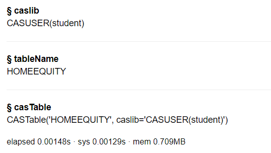
Let’s start by loading our data we saved in part 4 into CAS memory. I will load the sashdat file for my example. Use similar syntax to load the csv and parquet files.

conn.loadTable(path="homeequity_final.sashdat", caslib="casuser",
               casout={'name':'HomeEquity',
                               'caslib':'casuser', 'replace':True})

The home equity data is now loaded and ready for modeling.

Fit Random Forest

Before fitting a random forest in SAS Viya we need to load the decisionTree action set.

conn.loadActionSet('decisionTree')

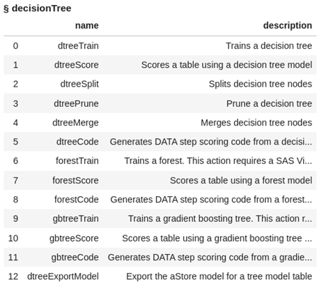
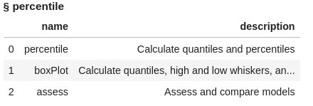
The decisionTree action set contains several actions, let’s display the actions to see what is available for us to use.

conn.help(actionSet='decisionTree')

This action set not only contains actions for fitting and scoring decision trees but also for fitting and scoring random forest models and gradient boosting models. Examples for fitting these decision trees are in Part 7 and examples for gradient boosting will be in the next post.

Fit a forest with the the forestTrain action on the HomeEquity training data set (i.e. where _PartInd_=1). Save the model to a file named rf_model and also to an astore format (more about this later in the post). Also, specify the nominal columns in a list, assign seed the value of 1234, and ask for the generation of variable importance information.

conn.decisionTree.forestTrain(
    table    = dict(name = 'HomeEquity', where = '_PartInd_ = 1'),
    target   = "Bad", 
    inputs   = ['LOAN' , 'IMP_REASON' , 'IMP_JOB' , 'REGION' , 'IMP_CLAGE' , 'IMP_CLNO' ,    
                       'IMP_DEBTINC' , 'IMP_DELINQ' , 'IMP_DEROG' , 'IMP_MORTDUE' , 'IMP_NINQ' ,  
                       'IMP_VALUE' , 'IMP_YOJ'], 
    nominals = ['BAD','IMP_REASON','IMP_JOB','REGION'],
    varImp=True,
    seed = 1234,
    casOut   = dict(name = 'rf_model', replace = True),
    saveState= dict(name = 'rf_astore', replace = True)
)

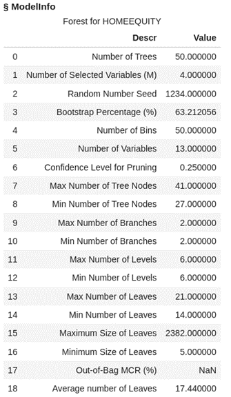
Looking at the output we can see that 50 trees were fit with 4 variables each, along with all the additional model info.

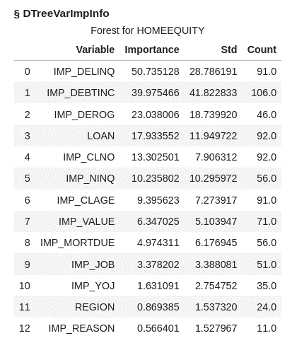
The variable importance table lists the variables in order of importance across all our tree models with imputed number of delinquent inquires as most important followed by imputed debt to income ratio.

Let’s take a look at the output tables currently in memory on the CAS server.

conn.table.tableInfo()

We have the Home Equity data we are using to fit our forest model, the model file (RF_MODEL), and the ASTORE (RF_ASTORE) file.

An ASTORE file is essentially a container for a trained analytical model. It stands for Analytic Store. This file stores all the necessary information about the model, including its parameters, coefficients, and other relevant data. Think of it as a packaged version of the model that can be easily deployed and used for making predictions on new data within the SAS Viya environment. It's like having a pre-built tool ready to apply to new situations without having to retrain the model each time.

Score Validation Data

In this post we will look at two ways to score data: using the ASTORE file and using the Model file. A third option, which will not be covered here, is creating a SAS Data Step score code using the forestCode action from the decisiontree action set.

ASTORE

First, score the validation data using the ASTORE file (RF_ASTORE). Using the head method you can see that the data is a binary representation.

conn.CASTable('rf_astore').head()

Before scoring the validation data using the ASTORE file in SAS Viya we need to load the aStore action set.

conn.loadActionSet('aStore')

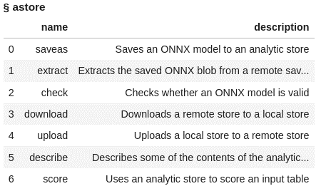
The actions included in the aStore actionset are listed below:

conn.builtins.help(actionSet='aStore')

Using the score action in the aStore action set, score the validation data from the home equity data file. Use _PartInd_ = 0 to identify the validation rows from the data. Create a new data set with the scored values named rf_astore_scored.

#Score the random forest model using the ASTORE
conn.aStore.score(
    table    = dict(name = 'HomeEquity', where = '_PartInd_ = 0'),
    rstore = "rf_astore",
    out = dict(name="rf_astore_scored", replace=True),
    copyVars = 'BAD'
)

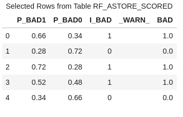
The new data set has 1788 rows and 5 columns.

Use the head method to view the first 5 columns of rf_astore_scored file.

conn.CASTable('rf_astore_scored').head()

In this data file, you'll find five columns, each serving a distinct purpose:

• P_BAD1: The predicted probability of an individual becoming delinquent on a home equity loan.
• P_BAD0: The complement of P_BAD1 (1 - P_BAD1), representing the predicted probability of an individual not becoming delinquent on a home equity loan.
• I_BAD: Here, you'll find the predicted classification value derived from the model.
• WARN_: Indicates why the model could not be applied because of things like missing values or invalid input values.
• BAD: This column represents our target variable, acting as the label or dependent variable (Y).

Model File

For the second method, lets score the validation data using in memory scoring table rf_model. First use the head method to look at the first five rows of data. Here you can see we have rows that represent each column used in fitting the forest model.

conn.CASTable('rf_model').head()

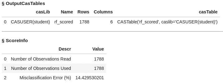
Now use rf_model and the forestScore action in the decsionTree action set to score the validation data (_PartInd_ = 0). Create a scored data table called rf_scored.

conn.decisionTree.forestScore(
    table    = dict(name = 'HomeEquity', where = '_PartInd_ = 0'),
    model = "rf_model",
    casout = dict(name="rf_scored",replace=True),
    copyVars = 'BAD',
    encodename = True,
    assessonerow = True
)

The data table rf_scored has 1788 rows and 6 columns. Output also includes the misclassification error at 14.4%

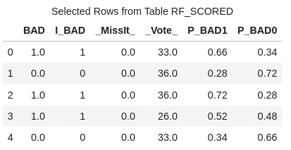
Use the head method to list the first 5 rows of rf_scored.

conn.CASTable('rf_scored').head()

In this data file, you'll find six columns, each serving a distinct purpose:

• BAD: This column represents our target variable, acting as the label or dependent variable (Y).
• I_BAD: Here, you'll find the predicted classification value derived from the model.
• MissIt: A value of 0 indicates a correct prediction, while 1 signifies an incorrect prediction when the scored data aligns with the observed target value.
• Vote: This column denotes the count of trees that accurately predict the value.
• P_BAD1: The predicted probability of an individual becoming delinquent on a home equity loan.
• P_BAD0: The complement of P_BAD1 (1 - P_BAD1), representing the predicted probability of an individual not becoming delinquent on a home equity loan.

Access Model

Next, we assess how well the forest model fits using the same metrics we used for logistic regression and decision trees: confusion matrix, misclassification rates and a ROC plot. We will use these measures to see how well our forest model fits the data and later use them to compare to other models.

To calculate these measures, we use the percentile action set and the assess action. First load the percentile action set and display the available actions.

conn.loadActionSet('percentile')
conn.builtins.help(actionSet='percentile')

We can use either of our scored data sets for doing assessment, as both have the same information and will give us the same output, so let’s use the rf_scored data created with the rf_model file above.

The access action creates two data sets named rf_assess and rf_assess_ROC.

conn.percentile.assess(
   table = "rf_scored",
   inputs = 'P_BAD1',
   casout = dict(name="rf_assess",replace=True),
   response = 'BAD',
   event = "1"
)

Using the fetch action list the first 5 rows of the rf_assess dataset for inspection. You can see the values at each of the depths of data from 5% incremented by 5.

display(conn.table.fetch(table='rf_assess', to=5))

Using the fetch action again on the rf_assess_ROC data, take a look at the first 5 rows. Here if we select cutoff of .03 the predicted true positives for our validation data would be 232 and true negatives 1219. Typically the default cutoff value is .5 or 50%.

conn.table.fetch(table='rf_assess_ROC', to=5)

Let’s bring the output data to the client as data frames to calculate the confusion matrix, misclassification rate, and ROC plot for the forest model.

rf_assess = conn.CASTable(name = "rf_assess").to_frame()
rf_assess_ROC = conn.CASTable(name = "rf_assess_ROC").to_frame()

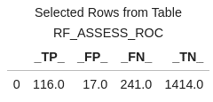
The confusion matrix is just a couple of quick calculations using the columns created in the rf_assess_ROC file.

The confusion matrix compares predicted values to actual values and gives a breakdown of the true positives, true negatives, false positives, and false negatives.

These measures help us evaluate the performance of the model and assess its accuracy in predicting the outcome of interest.

Use a cutoff value of 0.5, which means if the predicted probability is greater than or equal to 0.5 then our model predicts someone will be delinquent on their home equity loan. If the predicted value is less than 0.5 then our model predicts someone will not be delinquent on their home equity loan.

cutoff_index = round(rf_assess_ROC['_Cutoff_'],2)==0.5
conf_mat = rf_assess_ROC[cutoff_index].reset_index(drop=True)
conf_mat[['_TP_','_FP_','_FN_','_TN_']]

At the 0.5 cutoff value the true positives are 116 and the true negatives are 1414.

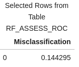
We can also do a quick calculation on the columns created for the confusion matrix to create the misclassification rate, which indicates how often the model makes an incorrect prediction.

conf_mat['Misclassification'] = 1-conf_mat['_ACC_']
miss = conf_mat[round(conf_mat['_Cutoff_'],2)==0.5][['Misclassification']]
miss

The misclassification rate of 14.4% matches the result obtained when we applied the rf_model to score the validation data

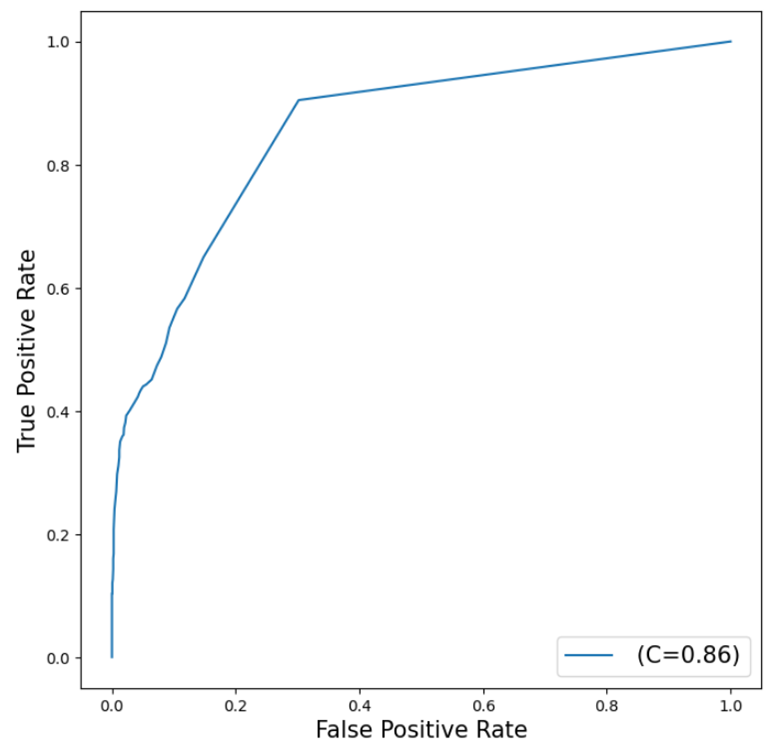
We'll create our final assessment metric in the form of a ROC (Receiver Operating Characteristic) Chart. This chart illustrates the trade-off between sensitivity and specificity, providing us with a comprehensive view of the forest model's performance. The curve's proximity to the top left corner indicates the model's overall performance, with closer positioning suggesting higher effectiveness.

Use the python package matplotlib to plot the ROC Curve.

from matplotlib import pyplot as plt
 
plt.figure(figsize=(8,8))
plt.plot()
 
plt.plot(rf_assess_ROC['_FPR_'],rf_assess_ROC['_Sensitivity_'], label=' (C=%0.2f)'%rf_assess_ROC['_C_'].mean())
 
plt.xlabel('False Positive Rate', fontsize=15)
plt.ylabel('True Positive Rate', fontsize=15)
plt.legend(loc='lower right', fontsize=15)
plt.show()

The curve generated by the forest model is reasonably close to the top left corner, suggesting that the model is fitting the data decently well, although there is still potential for improvement.

The value of C=0.86 represents the Area Under the Curve (AUC) statistic, which is another measure of fit. In this instance, our forest model outperforms a random classifier, which typically has an AUC of 0.5, but it falls short of the ideal scenario where the AUC equals 1, signifying a perfect model.

The Wrap-Up: Fitting a Random Forest Model

The Random Forest Model is easily fitted using the decisionTree action set, specifically with the forestTrain action, simplifying the process of creating such a model. Similarly, the forestScore action facilitates the scoring of holdout or new data with the forest model, enabling us to assess the overall effectiveness of the model.

In the next post, we will explore fitting a gradient boosting model with our dataset.

Related Resources

• SAS Help Center: Decision Tree Action Set
• SAS Help Center: forestTrain Action
• SAS Help Center: forestScore Action
• SAS Help Center: forestCode Action
• SAS Help Center: Percentile Action Set
• SAS Help Center: assess Action
• Getting Started with Python Integration to SAS® Viya® - Part 5 - Loading Server-Side Files into Memory