Public and private schools are struggling to figure out how to bring face-to-face instruction to students during this pandemic. Health risks to students and teachers, parents struggling with child-care options and/or support for virtual learning, and schools’ capacities and budget limitations make this problem a severe logistical challenge. Schools need to abide by CDC social distancing regulations as well as by each individual state’s guidance to minimize exposure and risk. In North Carolina, three different plans were considered by the state government:

Plan A: All students back to school with minimal social distancing
Plan B: Schools must limit the number of students and staff to ensure six feet of separation when stationary
Plan C: Remote-only learning

In July 2020, Governor Cooper announced guidance for all schools to operate under Plans B or C. On September 17th, he issued a statement allowing elementary schools to open under Plan A, reiterating that Plan A might not be right for all schools and each district is in control of their reopening plan.

Most school districts are considering Plan B, which presents specific challenges to school administrators. One of the challenges is to find the best possible schedule for groups of students assigned to classrooms and matching teachers to those groups such that state and federal mandates are respected. Given the number of possible combinations of schedules, this is not a trivial problem to solve. Fortunately, operations research is the best analytical tool to support decision makers with data insights and scenario recommendations for this case.

In this article, we consider Plan B and propose a mixed integer linear programming (MILP) model that maximizes the number of student hours of in-class instruction, given restricted room capacities due to social distancing requirements.

Problem Description

In this section, we describe the structure of the problem. Let $S = \{1,2,\dots,\text{n}_{S}\}$ be the set of schools in a school district. The set of schools includes elementary, middle, and high school grade levels in that school district. We assume that the students are not transferrable between schools and the schools do not share room spaces. Thus, the optimization model can be defined independently of the school index and is executed in parallel for the schools in $S$ . Let $G = \{1,2,\dots,\text{n}_{G}\}$ be the set of grades, and $R = \{1,2,\dots,\text{n}_{R}\}$ be the set of rooms in a school $s \in S$ . Due to the social distancing requirement, the rooms have a maximum occupancy restriction that is lower than its original capacity. Let $\text{capacity}_{r}$ be the restricted capacity of room $r \in R$ , and let $\text{population}_{g}$ be the number of students enrolled in grade $g \in G$ .

The scheduling time horizon is divided into time blocks $B = \{1,2,\dots,\text{n}_{B}\}$ . We consider three different time horizon scenarios (all under Plan B): monthly rotating, weekly rotating, and daily rotating. Figure 1 shows the different time horizon scenarios. Under the monthly rotation scenario, students attend full day school during certain weeks of a month and do remote learning for the rest of the time. For example (as shown in Figure 1 below), 1^st grade might be scheduled to come on the third and fourth week of each month. Under the weekly rotation scenario, students attend full day school during certain days of a week, every week. For example, 3^rd grade might be scheduled to come to school on Tuesdays and Thursdays. Under the daily rotation scenario, students attend school daily, but for a predefined block of time. For example, 5^th grade might be scheduled to attend school between 8 and 10am each day.

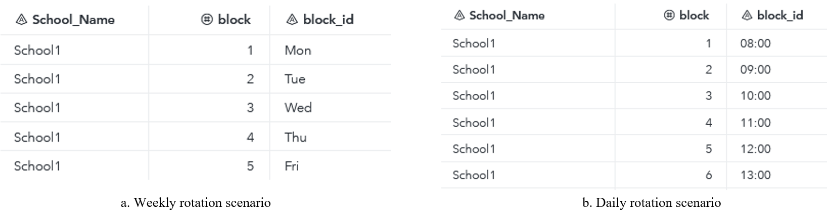
The set $B$ of time blocks for monthly, weekly, and daily plans are defined as {Week1, Week2, Week3, Week4}, {Monday, Tuesday, Wednesday, Thursday, Friday}, and {8am, 9am, 10am, 11am, 12pm, 1pm}, respectively. Let $\text{duration}_{b}$ be the duration of each time block $b \in B$ . In this study, we set $\text{duration}_{b}$ to be 1. It is defined as a parameter to give flexibility for the user to change if needed.

The proposed model is developed to create a schedule by assigning students in grades to time blocks and rooms. The following assumptions are considered in the development of the proposed model:

Students in a grade cannot be split between time blocks. If a grade $g$ is assigned to a time block $b$ , then all the students in that grade $g \ \text{(population}_{g}\text{)}$ should be accommodated in time block $b$ .
Each grade in a school $s$ should attend an equal number of time blocks. Say, in an elementary school, if 1^st grade attends two time blocks, then all other grades (K, 2^nd-5^th grades) should attend two time blocks.
In the daily rotation scenario, the assignment of time blocks for grades should be consecutive as transportation of students multiple times a day is not feasible.
Under the daily rotation scenario, a common break or transition time is added to the schedule to enable transportation, cleaning/sanitation of classrooms, other logistics, etc. Let $\text{transitionwindow}$ be the transition time, defined in number of time blocks, in the daily rotation.
A fraction of students, denoted by $\text{virtualpercent}$ , attend full online / remote learning sessions. This fraction of students is not included in the scheduling.

Input Data

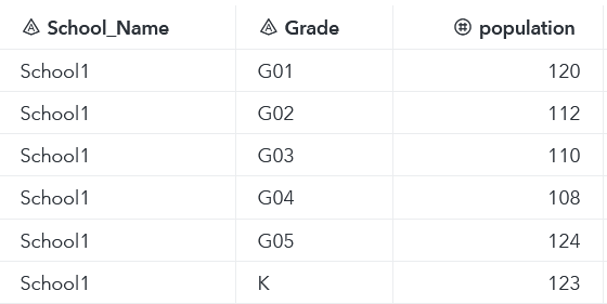
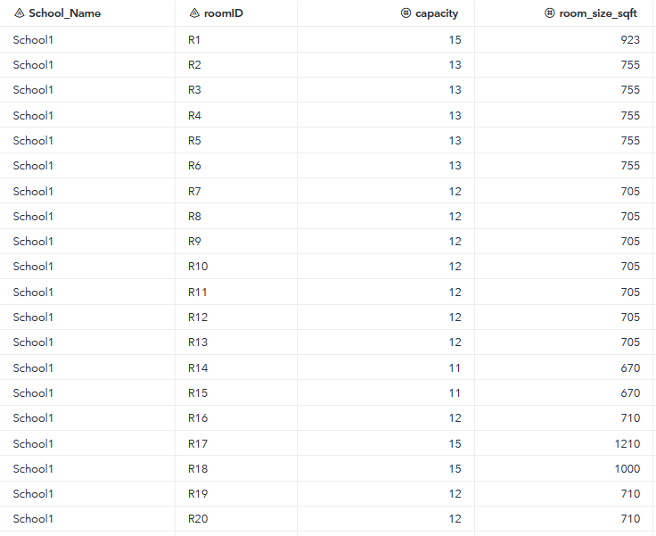
This section describes the input data tables required for the optimization model. The input data include three tables: the schools table, the rooms table, and the time blocks table. The schools table contains the population (enrollment) data for each grade at the school. The rooms table contains data on the rooms available in the school along with its restricted capacity (capacity column) and room size (room_size_sqft column).

Figures 2 and 3 shows sample school and room data for an elementary school (School1). We can use the restricted capacity from the capacity column or we can calculate it using the room size and square feet per student guideline. For example, suppose you want to analyze a scenario with 60 square feet per student. In the sample data (Figure 3), room R1 is 923 square feet and can accommodate $\lfloor 923 / 60\rfloor = 15$ students.

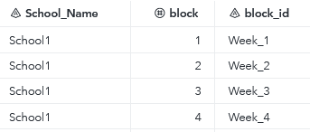
The data in the time blocks table depend on the selection of the time horizon scenario. Figure 4 shows a time blocks table for the monthly rotation scenario. It has four time blocks: {Week_1, Week_2, Week_3, Week_4}.

Figures 5 (a) and (b) show the time blocks tables for the weekly and daily rotation scenarios, respectively.

Figure 5: Weekly and Daily rotation scenarios

Model Formulation

Considering the student enrollment, and a finite number of rooms with restricted capacity, the problem can be formulated as a mixed integer linear programming (MILP) model, where the objective is to maximize the in-person instructional hours for the students. The decision variables for the model are shown below:

Decision Variables

$\text{NumStudents}_{g, r, b} \ge 0$ is the number of students in grade $g$ , room $r$ , and time block $b$
$\text{AssignGrRmBl}_{g,r,b} \in \{0,1\}$ is a binary variable indicating if room $r$ is in use at time block $b$ for grade $g$
$\text{AssignGrBl}_{g,b} \in \{0,1\}$ is a binary variable indicating if grade $g$ is assigned to time block $b$
$\text{AssignGrRm}_{g,r} \in \{0,1\}$ is a binary variable indicating if grade $g$ is assigned to room $r$
$\text{AvgNumStudents} \ge 0$ is the average number of student hours per time block in any grade
$\text{ConsecutiveGrBl}_{g,b} \in \{0,1\}$ is a binary variable indicating if block $b$ is the starting time block for grade $g$
Note that $\text{ConsecutiveGrBl}_{g,b}$ is used only in the daily rotation scenario where assignment of time blocks for grades must be consecutive.

Objective Function

The objective function $\text{(M1)}$ is to maximize the instructional hours for the students and can be written as:

$\text{(M1) maximize TotalStudentHours}=\sum\limits_{g,r,b} \text{duration}_b \ \text{NumStudents}_{g,r,b}$

Constraints

Constraint (1) is the room capacity constraint. This constraint ensures that the number of students in grade $g$ assigned to room $r$ in time block $b$ should not exceed the capacity of the room $r$ . Recall that the capacity of each room has already been modified to allow for social distancing restrictions. When $\text{AssignGrRmBl}_{g,r,b}$ is zero, the right-hand side of the constraint becomes zero and forces $\text{NumStudents}_{g, r, b}$ to be zero.

$\text{NumStudents}_{g,r,b} \leq \text{capacity}_r \ \text{AssignGrRmBl}_{g,r,b} \quad \forall~g,r,b$ $\text{(1)}$

The room block assignment constraint (2) ensures that a room $r$ in time block $b$ should be assigned to at most one grade.

$\sum_{g} \text{AssignGrRmBl}_{g,r,b} \leq 1 \quad \forall~r,b$ $\text{(2)}$

Constraint (3) ensures that the number of students assigned in a grade $g$ and time block $b$ across all rooms should be equal to the enrollment $(\text{population}_{g})$ in that grade attending in-class instruction.

$\sum_r \text{NumStudents}_{g,r,b} = (1 - \text{virtualpercent}) \ \times \ \text{population}_{g} \ \times \ \text{AssignGrBl}_{g,b} \quad \forall~g,b$ $\text{(3)}$

Constraint (4) ensures that the average number of student hours per block in a grade $g$ is the same across all grades.

$\sum_{r,b} \frac{\text{NumStudents}_{g,r,b}}{\text{n}_{b} \ \times \ \text{population}_{g} \ \times \ (1-\text{virtualpercent})} = \text{AvgNumStudents} \quad \forall~g$ $\text{(4)}$

Constraints (5) and (6) compute grade-block assignment and grade-room assignment variables from the grade, room, and block assignment variable.

$\text{AssignGrRmBl}_{g,r,b} \leq \text{AssignGrBl}_{g,b} \quad \forall~g,r,b$ $\text{(5)}$

$\text{AssignGrRmBl}_{g,r,b} \leq \text{AssignGrRm}_{g,r} \quad \forall~g,r,b$ $\text{(6)}$

Constraints specific to the daily rotation scenario

When students are scheduled to attend part-day classes, the constraints (7) through (11) ensure that the students in a grade $g$ are assigned to consecutive time blocks.

$\text{ConsecutiveGrBl}_{g,1} = \text{AssignGrBl}_{g,1} \quad \forall~g$ $\text{(7)}$

$\text{ConsecutiveGrBl}_{g,b} \geq \text{AssignGrBl}_{g,b} - \text{AssignGrBl}_{g,b-1} \quad \forall~g, b \in \{2,\dots,\text{n}_{B}\}$ $\text{(8)}$

$\sum_{b} \text{ConsecutiveGrBl}_{g,b} \leq 1 \quad \forall~g$ $\text{(9)}$

$\text{ConsecutiveGrBl}_{g,b} \leq \text{AssignGrBl}_{g,b} \quad \forall~g,b \in \{2,\dots,\text{n}_{B}\}$ $\text{(10)}$

$\text{ConsecutiveGrBl}_{g,b} \leq 1 - \text{AssignGrBl}_{g,b-1} \quad \forall~g,b \in \{2,\dots,\text{n}_{B}\}$ $\text{(11)}$

Constraint (12) ensures that there is a break for $\text{transitionwindow}$ time blocks for cleaning and/or transportation.

$\text{AssignGrBl}_{g1, b-\text{transitionwindow}} \leq 1- \text{ConsecutiveGrBl}_{g,b} \quad \forall~g,g1 \in G, \text{and } b \in \{1+\text{transitionwindow},\dots,\text{n}_{B}\}$ $\text{(12)}$

We will now discuss an optional constraint that tightens constraint (12) and improves computational time of the model. Let $Q = \{1,2,\dots,\text{n}_{G}\}$ be the reordered set of grades, where $\text{population}_{1} \leq \text{population}_{2} \le \dots \leq \text{population}_{n_{G}}$ . Let $\text{cum_population}_{q}= \sum_{i=1}^{q} \text{population}_{i}$ be the cumulative sum of enrollments for the smallest $q$ grades. Let $\text{totcapacity}$ be the total capacity of the school across all rooms. Let $\text{MaxGradesBlock} = \text{max} \{q \in \text{Q: } \text{cum_population}_{q} \leq \text{totcapacity} \}$ be the maximum number of grades in a time block. Constraint (13) ensures that no grades are assigned to the break period.

$\sum_{g1 \in G} \text{AssignGrBl}_{g1, b-\text{transitionwindow}} \leq \text{MaxGradesBlock} \ \times \ (1- \text{ConsecutiveGrBl}_{g,b}) \quad \forall~g,b \in \{1+\text{transitionwindow},\dots,\text{n}_{B}\}$ $\text{(13)}$

Constraints (14) and (15) ensure that the students assigned to room $r$ in grade $g$ do not change rooms. There is no reason for a grade to switch rooms during the day, because room capacities per time block and number of students per grade are constant. These constraints force grades to stay in the same rooms once they have been assigned. Note that the constraint (14), which ensures students to stay in the same room, is valid only if the $\text{transitionwindow}$ is at least one period. If the $\text{transitionwindow}$ is zero, it might be optimal to move students to a different room in a time block when a new grade is starting.

$\text{AssignGrRmBl}_{g,r,b} + 1 \geq \text{AssignGrBl}_{g,b} + \text{AssignGrRm}_{g,r} \quad \forall~g,r,b$ $\text{(14)}$

$\text{AssignGrRmBl}_{g,r,b} \leq \text{NumStudents}_{g,r,b} \quad \forall~g,r,b$ $\text{(15)}$

Special case

When solving for the daily rotation scenario and $\text{transitionwindow}$ = 0, the assigned time blocks for two grades can overlap. For example, in the optimal solution 1^st grade could attend school between 8am - 11am and 2^nd grade could attend between 10am - 1pm. It might be beneficial for 1^st grade students to change rooms at 10am in order to accommodate the 2^nd grade. Therefore, when solving the daily rotation scenario and $\text{transitionwindow}$ = 0, we drop constraints (12) and (13) because they are not relevant, and we drop constraint (14) because we want to allow students to change rooms. We also add a secondary objective $\text{(M2)}$ to minimize the number of room changes across all grades.

$\text{(M2) minimize RoomChanges}=\sum\limits_{g,r} \text{AssignGrRm}_{g,r}$

We solve a bi-criteria problem using a sequential approach – solve first for (M1), and then solve for (M2) with a constraint on (M1). Let $\text{primary_objective_value}$ be the objective value obtained when solving for (M1). Constraint (16) is added when we solve for minimizing room changes (M2):

$\sum\limits_{g,r,b} \text{duration}_{b} \ \text{NumStudents}_{g,r,b} \geq \text{primary_objective_value}$ $\text{(16)}$

Solving the Model

The model is coded and solved using the runOptmodel CAS action in SAS Optimization. We start by defining the index sets, parameters, and read data into the index sets and parameters by using the READ DATA statements. The decision variables are then declared by using the index sets.

proc cas;
   loadactionset 'optimization';
   run;
   source pgm;
 
   /*************************************************/
   /* Define sets                                   */
   /*************************************************/
   set <str> ROOMS;
   set <str> GRADES;
   set <num> BLOCKS;
 
   /*************************************************/
   /* Define inputs                                 */
   /*************************************************/
   str block_id {BLOCKS};
   num duration {BLOCKS};
   num capacity {ROOMS};
   num population {GRADES};
 
   /*************************************************/
   /* Read data                                     */
   /*************************************************/
   read data &caslib..input_room_data into ROOMS=[roomID] capacity;
   read data &caslib..input_school_data into GRADES=[grade] population; 
   read data &caslib..input_block_data into BLOCKS=[block] block_id duration;
 
   /*************************************************/
   /* Decision Variables                            */
   /*************************************************/
   var NumStudents {GRADES, ROOMS, BLOCKS} >= 0;
   var AssignGrRmBl {GRADES, ROOMS, BLOCKS} binary;
   var AssignGrBl {GRADES, BLOCKS} binary;
   var AssignGrRm {GRADES, ROOMS} binary;
   var AvgNumStudents >= 0;
   var ConsecutiveGrBl {GRADES, BLOCKS} binary;

The parameters needed to compute maxGradesinBlock are calculated in a DATA step prior to calling PROC CAS. As discussed, the maxGradesinBlock parameter is used in constraint (13) to improve the computation time.

   /* Number of grades in a block */ 
   num totcapacity = sum {r in ROOMS} capacity[r];
   num cum_population{GRADES};
   num grade_count{GRADES};
 
   read data &caslib..output_grades_in_block into [grade] cum_population grade_count;
   num maxGradesinBlock = max {q in GRADES: cum_population[q] <= totcapacity} grade_count[q];

The objective of the problem is to maximize the instructional hours for the students and is written as follows:

   /*************************************************/
   /* Objective Functions                           */
   /*************************************************/
   /* Objective function returns the total student hours (weighted by duration of the block) in the classroom */
   max TotalStudentsHours = sum {g in GRADES, r in ROOMS, b in BLOCKS} duration[b] * NumStudents[g, r, b];

The RoomChanges objective function is used only under the special case and is written as follows:

   /* Adding a small penalty for choosing different rooms */
   min RoomChanges = sum {g in GRADES, r in ROOMS} AssignGrRm[g, r];

Next, we show the sets of constraints in the model. The constraints are shown in the order discussed in the model formulation section. As you can observe, both $\text{virtualpercent}$ and $\text{transitionwindow}$ parameters are defined as macro variables ( $\text{virtual_percent}$ , $\text{transition_window}$ ) and can be modified by the user.

   /*************************************************/
   /* Constraints                                   */
   /*************************************************/
   /********************* Room Capacity related constraints *********************/  
   /* Students assigned to a grade,block,room should not exceed the capacity the room. */
   con GradeRoomBlockAssignment {g in GRADES, r in ROOMS, b in BLOCKS}:
      NumStudents[g, r, b] <= capacity[r] * AssignGrRmBl[g, r, b];
 
   /* Room/block assigned to a grade should be less than or equal to 1. - A room can be assigned to a max. of one grade in a time block */
   con RoomBlockAssignment {r in ROOMS, b in BLOCKS}:
      sum {g in GRADES} AssignGrRmBl[g, r, b] <= 1;
 
   /********************* Number of students constraints *********************/  
   /* Number of students in a grade, block across all rooms should be equal to the population in that grade */
   con GradePop {g in GRADES, b in BLOCKS}:
      sum {r in ROOMS} NumStudents[g, r, b] = (1 - (&virtual_percent. / 100)) * population[g] * AssignGrBl[g, b];
 
   /********************* Student Equality constraints *********************/  
   /* Computing average number students attending in a grade and Ensuring that the AvgNumStu is same across all grades*/
   con GradeAvg {g in GRADES}:  
      sum {r in ROOMS, b in BLOCKS} NumStudents[g, r, b] / (card(BLOCKS)* population[g] * (1 - (&virtual_percent. / 100))) = AvgNumStudents;
 
   /********************* Deriving Grade-Block and Grade-Room variables constraints **********************/  
   /* Deducing grade, block assignment from grade,block,room assignment. */
   con GradeBlockAssignment {g in GRADES, r in ROOMS, b in BLOCKS}:
      AssignGrRmBl[g, r, b] <= AssignGrBl[g, b];
 
   /* Deducing grade, room assignment from grade,block,room assignment. */
   con GradeRoomAssignment {g in GRADES, r in ROOMS, b in BLOCKS}:
      AssignGrRmBl[g, r, b] <= AssignGrRm[g, r];
 
   /********************* Constraints specific to Plan 4 *********************/
   /* Constraint that ensures a grade is assigned only to continuous blocks */
   con ConsFirstBlock {g in GRADES}:
      ConsecutiveGrBl[g, 1] = AssignGrBl[g, 1];
 
   con ConsPattern {g in GRADES, b in 2..card(BLOCKS)}:
      ConsecutiveGrBl[g, b] >= AssignGrBl[g, b] - AssignGrBl[g, b-1];
 
   con ConsPatternRes {g in GRADES}:
      sum {b in BLOCKS} ConsecutiveGrBl[g, b] <= 1;
 
   /* If grade g is assigned to block b-1 or if grade g is not assigned to block b, then force ConsecutiveGrBl[g, b] to be 0 */
   con ConsAddCuts {g in GRADES, b in 2..card(BLOCKS)}:
      ConsecutiveGrBl[g, b] <= AssignGrBl[g, b];
 
   con ConsAddCuts1 {g in GRADES, b in 2..card(BLOCKS)}:
      ConsecutiveGrBl[g, b] <= 1 - AssignGrBl[g, b-1];
 
   /* Breaks in between for cleaning */
   con Breakconstraint {g in GRADES, g1 in GRADES, b in (1+&transition_window.) ..card(BLOCKS)}:
      AssignGrBl[g1, (b-&transition_window.)] <= 1 - ConsecutiveGrBl[g, b];
 
   con Breakconstraint1 {g in GRADES, b in (1+&transition_window.) ..card(BLOCKS)}:
      sum {g1 in GRADES} AssignGrBl[g1, (b-&transition_window.)] <= maxGradesinBlock * (1 - ConsecutiveGrBl[g, b]);
 
   /* Constraint that ensures students assigned to a room r in a grade g does not change rooms */
   con NoRoomChanges {g in GRADES, r in ROOMS, b in BLOCKS}:
      AssignGrRmBl[g, r, b] + 1 >= AssignGrBl[g, b] + AssignGrRm[g, r];
 
   con NoRoomChanges2 {g in GRADES, r in ROOMS, b in BLOCKS}:
      AssignGrRmBl[g, r, b] <= NumStudents[g, r, b];
 
   /* Constrain each of the objective functions to prevent worse solutions */
   num primary_objective_value init 0;
 
   con PrimaryObjConstraint:
      sum {g in GRADES, r in ROOMS, b in BLOCKS} duration[b] * NumStudents[g, r, b] >= primary_objective_value;

Next, we discuss the solve statements. We have two solve cases: one for the monthly and weekly rotation scenarios and the other for the daily rotation scenario. The plan_num macro variable is used to define the rotation scenario: plan_num=2 is the monthly rotation scenario, plan_num=3 is the weekly rotation scenario, and plan_num=4 is the daily rotation scenario. For the monthly and weekly rotation scenarios, we drop the constraints that are specific to the daily rotation scenario.
In the special case of daily rotation scenario with $\text{transitionwindow}$ =0, we drop the constraints named Breakconstraint, Breakconstraint1, and NoRoomChanges. We also solve for objective $\text{M2}$ ( $\text{minimize RoomChanges}$ ), given the optimal value of objective $\text{M1}$ ( $\text{maximize TotalStudentHours}$ ) is preserved.

We are using the MILP solver to solve the problem, allowing a relative objective gap of 1%.

   /*************************************************/
   /* Solve                                         */
   /*************************************************/
   if &plan_num. = 2 or &plan_num. = 3 then do;
      drop Breakconstraint;
      drop Breakconstraint1;
      drop ConsFirstBlock;
      drop ConsPattern;
      drop ConsPatternRes;
      drop ConsAddCuts;
      drop ConsAddCuts1;
      drop NoRoomChanges;
      drop PrimaryObjConstraint;
 
      solve obj TotalStudentsHours with milp / loglevel=3 relobjgap=0.01;  
   end;
 
   if &plan_num. = 4 then do;
      drop PrimaryObjConstraint;
 
      if &transition_window. = 0 then do;
         drop Breakconstraint; 
         drop Breakconstraint1;
         drop NoRoomChanges;
      end;
 
      solve obj TotalStudentsHours with milp / loglevel=3 relobjgap=0.01;
 
      /* Cleaning step - before primalin */
      for {g in GRADES, r in ROOMS, b in BLOCKS} AssignGrRmBl[g, r, b] = round(AssignGrRmBl[g, r, b]);
      for {g in GRADES, b in BLOCKS} AssignGrBl[g, b] = round(AssignGrBl[g, b]);
      for {g in GRADES, r in ROOMS} AssignGrRm[g, r] = round(AssignGrRm[g, r]);
      for {g in GRADES, b in BLOCKS} ConsecutiveGrBl[g, b] = round(ConsecutiveGrBl[g, b]);
 
      if &transition_window. = 0 then do;
         /* Solve for secondary objective only if primary objective solve was successful */
         if _NSOL_ > 0 then
            do;
            primary_objective_value = TotalStudentsHours.sol;
            restore PrimaryObjConstraint;
            solve obj RoomChanges with milp / primalin loglevel=3 relobjgap=0.01;
         end;
      end;
   end;

After we solve the problem, we use a CREATE DATA statement to create the output table with all the required data for the output visualization. As mentioned previously, the optimization model can be run independent of the school index and can be executed in parallel for the schools in $S$ (i.e., for the entire school district). We use the groupBy option in the runOptmodel statement to execute the model for multiple schools in parallel. Note that if the input data have only school, the runOptmodel statement is still relevant and is executed for that one school. The nGroupByTasks = ‘ALL’ option in the runOptmodel statement enables the model to use all the threads on each worker node when optimizing the BY groups in parallel.

   /*************************************************/
   /* Create output data                            */
   /*************************************************/
   num total_capacity = 6 * sum {r in ROOMS} capacity[r];
   num total_population = sum {g in GRADES} population[g];
   num StudentHoursDay = (TotalStudentsHours.sol * 6) / card(BLOCKS);
   num AvgHoursPerStuWeek = (StudentHoursDay*5) / total_population;
   num totHoursStuWeek = (StudentHoursDay*5);
   num num_blocks_scen = card(BLOCKS);
 
   num num_students {g in GRADES, r in ROOMS, b in BLOCKS} = round(NumStudents[g,r,b].sol);
   num grade_room_block_assignment {g in GRADES, r in ROOMS, b in BLOCKS} = round(AssignGrRmBl[g,r,b].sol);
   num AssignGrBlSol {g in GRADES, b in BLOCKS} = round(AssignGrBl[g,b].sol);
 
   create data &caslib..output_full_assignment from [grade roomID block] = {g in GRADES, r in ROOMS, b in BLOCKS} 
      num_students 
      grade_room_block_assignment
      AssignGrBl = AssignGrBlSol[g,b]
      block_id[b] 
      duration[b] 
      population[g]
      capacity[r]
      total_capacity
      StudentHoursDay
      AvgHoursPerStuWeek
      num_blocks_scen
      total_population
      totHoursStuWeek;
 
   endsource;
   runOptmodel / code=pgm groupBy='School_Name' nGroupByTasks='ALL';
   run;
quit;

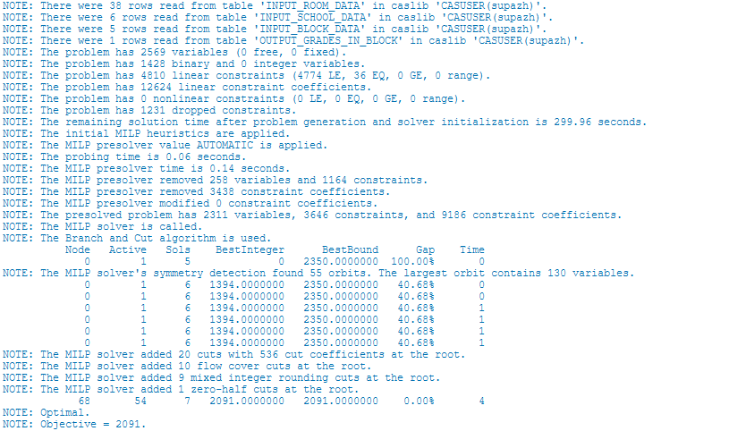
Figure 6 shows the optimization log from executing the model for an elementary school under the weekly rotation scenario. The data for this problem are available in GitHub. First, the optimization log shows the details of this problem instance such as the numbers of variables and constraints, before and after the presolver step.. Next, you can see the iteration log with information about each iteration until convergence criteria are reached (we specified a relative objective gap of 1%). For this problem instance, the solver was able to find an optimal solution of 2091 student hours in 4 seconds of run time.

Visualizing the Output

To begin analyzing solutions and options for a full school district, we wanted to compare the relevant KPIs such as average weekly in-person instructional hours per student, average room utilization, and teacher workload. We ran the optimization engine described above for the three rotation scenarios (monthly, weekly, and daily) and for different capacity settings (measured as minimum square footage per student). Figure 7 displays the results of these optimization runs. We used SAS Visual Analytics to build user-friendly visual representations. Note: These results have been fully anonymized and do not represent any specific school or school district.

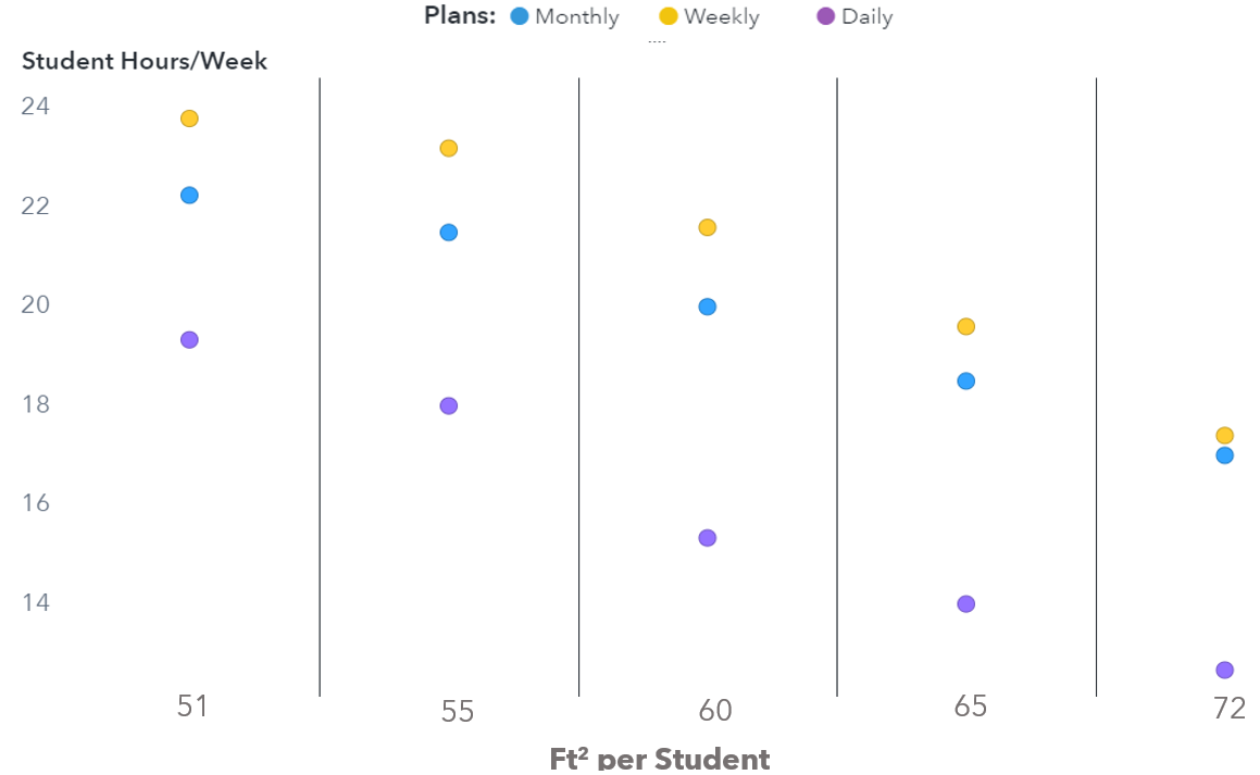
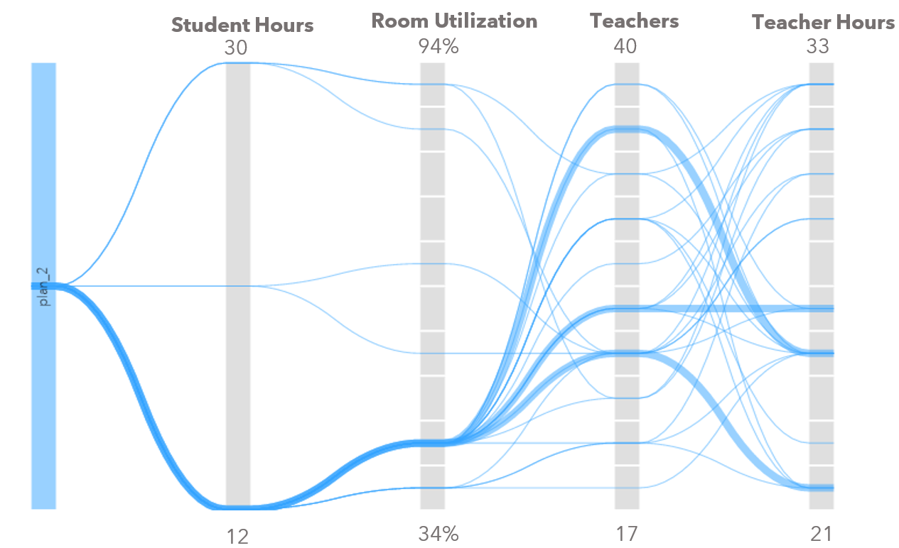
Figure 7: Minimum square footage per student vs. student hours per week

In most capacity settings, the weekly rotation outperforms the other scenarios, meaning we are able to deliver more in-person instructional hours while satisfying capacity constraints and better utilizing the limited room availability. Figure 8 shows the scenario for a weekly rotation and 60 square feet per student. Most schools can only accommodate an average of 12 weekly in-person instructional hours while a few schools can accommodate as high as 30 hours. The number of required teachers to generate this schedule has a wider distribution across all schools, varying from 17 to 40. The numbers of hours a teacher works per week varies between 21 and 33.

Figure 8: KPIs for weekly rotation scenario and 60 square feet per student

Once the school administrators choose a time-horizon plan and the social distancing guideline, we can then drill down into recommend detailed student schedule and classroom assignments. Figure 9 shows the grade and time block schedule for one elementary school under the monthly rotation scenario. In this example, K and 5^th grade students attend in-person instruction in weeks 1 and 2; 1^st, 2^nd, 3^rd, and 4^th grade students come to school in weeks 3 and 4.

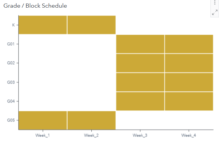
Figure 10 shows the grade, room, and time block assignment schedule for students. The blue dots in the chart represent the room number where the students are assigned in the corresponding time block.

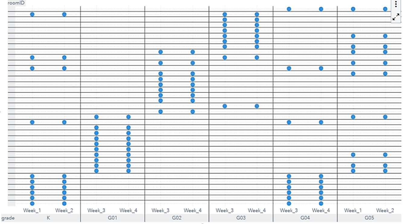
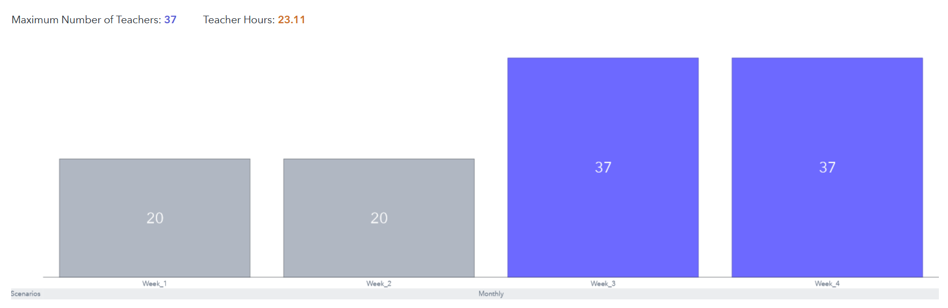
Figure 10: Grade, room, time block schedule

Figure 11 shows the number of teachers required at the school by time block. In this example, the school needs 20 teachers in weeks 1 and 2, and 37 teachers in weeks 3 and 4.

Figure 11: Number of teachers by time block

Summary

This article addresses an important and relevant problem of reopening schools and safely bringing students back to in-class instruction. Given a finite number of rooms and maximum occupancy restrictions, this study proposes an optimal schedule to get students back to school in order to maximize the in-person instructional hours of students. The optimization problem is modeled as a mixed integer linear programming model and solved using the runOptmodel action in SAS Optimization. We use realistic data from a school district and execute the model for different time horizon scenarios and capacity settings. We also developed visualizations using SAS Visual Analytics to aggregate and analyze the results from the runs. For a desired scenario, SAS Visual Analytics reports can be used to drill down into detailed schedules for students, classrooms, and teachers. This model supports school administrators in making analytics-based decisions for safely bringing students back to classrooms. We are eager to partner with school organizations to share these insights and potentially aid their decision planning during these challenging times.

Acknowledgments

The author would like to thank Michelle Opp, Rob Pratt, Natalia Summerville, and Matt Fletcher for their contributions to the model formulation and the blog content.

Additional reading

A high level description of the problem can be found in the Mathematical Optimization to Support Safe Back-to-School LinkedIn article.

Code

The code and data for this problem are available in GitHub at
https://github.com/sascommunities/sas-optimization-blog/tree/master/back_to_school_optimization.

Blogs