Last week I was visiting San Diego for the SANDS conference.  I always enjoy this conference as I get to interact closely with the users to hear of their pains and innovative solutions to creating Clinical Graphs.

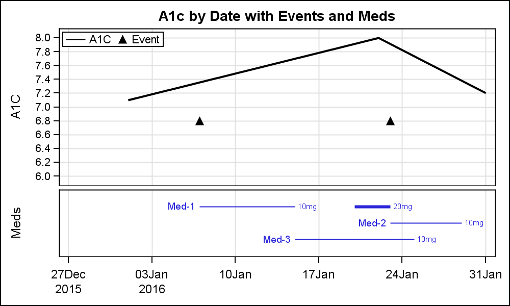
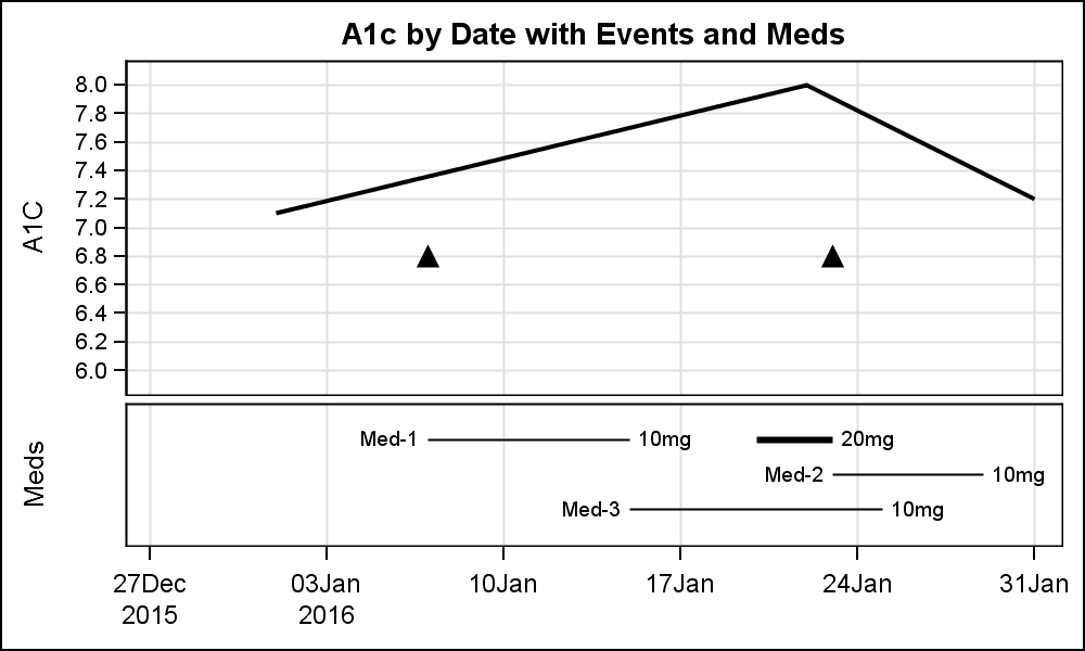In the conference Ed Barber asked about displaying A1c data along with some events data on a time line, along with data showing the meds that were used in the same graph as shown on the right.  Click on the graph for a higher resolution image.

As always, I like to break down the desired result into component parts, and then use the appropriate statement combinations to create the graph.  In this case, the graph is really in two parts.  The upper cell has a display of the subject A1c by date, along with markers to show the occurrence of some adverse events by date.

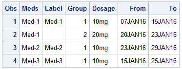
The lower cell contains a graph of the medications and their duration, along with the dosage represented as the thickness of the line.  The data for this is most ideally coded as columns with medicine name, dosage and start and end dates for the duration.

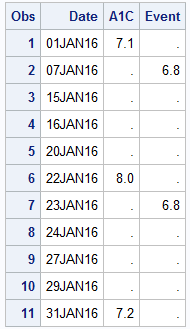
The easiest way to get the data in one data set (as needed to graph it), I create each data set separately as shown below.

 

 

 

 

 

 

 

 

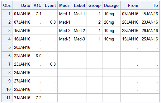Then, I do a simple merge to get one data set as shown on the right.

Now, we can plot the curve showing A1c x Date and overlay a scatter plot of Event x Date, where "Event" column contains the y-axis value for plotting the marker.  In this case, I have used a value that will put it somewhere in the range of the A1c data.

For the plot in the bottom cell, we can use a HighLow plot to display the start and end dates for each medication.  We can also display the med name as a LowLabel and the dosage as the HighLabel to produce the graph shown at the top.

Note, I have used a GTL template to create a 2-cell graph, with a common x-axis.  While the GTL code is more verbose, the structure of the graph is quite simple.  We use a 2-row LAYOUT LATTICE, and populate each cell with a LAYOUT OVERLAY.  The upper container has a Series and a Scatter plot, while the lower cell has one HighLow plot.

Note the use of the DATTRMAP data set for setting the attributes of the HighLow plot line by group.  Group=2 has the thicker line.

GTL Template code:

proc template;
  define statgraph A1c_1;
    begingraph;
      entrytitle 'A1c by Date with Events and Meds';
      layout lattice / rows=2 columndatarange=union rowweights=(0.7 0.3) rowgutter=5px;
        columnaxes;
          columnaxis / griddisplay=on display=(ticks tickvalues);
        endcolumnaxes;

        layout overlay / yaxisopts=(griddisplay=on tickvalueattrs=(size=8)
                     linearopts=(viewmin=6 tickvaluesequence=(start=6 end=8 increment=0.2)));
          seriesplot x=date y=a1c / lineattrs=(thickness=2);
          scatterplot x=date y=event / markerattrs=(symbol=trianglefilled size=12);
       endlayout;

        layout overlay / yaxisopts=(display=(label) reverse=true);
          highlowplot y=meds low=from high=to / group=group lowlabel=label highlabel=dosage
                      lineattrs=(color=black) labelattrs=(color=black);
        endlayout;
      endlayout;
    endgraph;
  end;
run;

proc sgrender data=both template=a1c_1 dattrmap=attrmap;
  dattrvar group='Meds';
run;

The graph on the right uses two HIGHLOW plot statements to differentiate the display of the Dosage from the Meds.  Click on the graph for a higher resolution image.  The HIGHLOW plot has only one option for LabelAttrs, which applies to both the low and high labels.  So, to display the HighLabel using different label settings, I one HighLow plot with LowLabel only, and one HighLow plot with HighLabel only with LabelAttrs.  The line thickness for 2nd plot is made zero.

Once you understand the structure of the graph, you can create a 2-cell graph using SG by splitting the height of the graph using the y-axis and y2-axis sections as shown below.

SG code:

title 'A1c by Date with Events and Meds';
proc sgplot data=both noautolegend dattrmap=attrmap;
series x=date y=a1c / lineattrs=(thickness=2);
scatter x=date y=event / markerattrs=(symbol=trianglefilled size=12);
refline 5.8 / noclip;
highlow y=meds low=from high=to / y2axis group=group attrid=Meds
lowlabel=label labelattrs=(color=black) lineattrs=(color=black);
highlow y=meds low=from high=to / y2axis group=group attrid=Meds
highlabel=dosage labelattrs=(color=gray size=6) lineattrs=(thickness=0);
yaxis offsetmin=0.3 offsetmax=0.05 values=(6 to 8 by 0.2) min=5.8 max=8 valueshint
label='A1c' labelpos=datacenter valueattrs=(size=8) grid;
y2axis offsetmin=0.75 offsetmax=0.07 display=none reverse;
xaxis display=(nolabel) grid;
run;

Update:  Recently a co-worker suggested that a legend would help to decode the information.  Now, a legend is added in the upper cell, as shown in the graph on the right.  Also, the lines representing the "Meds" are made blue, to distinguish from the A1c curve.

 

 

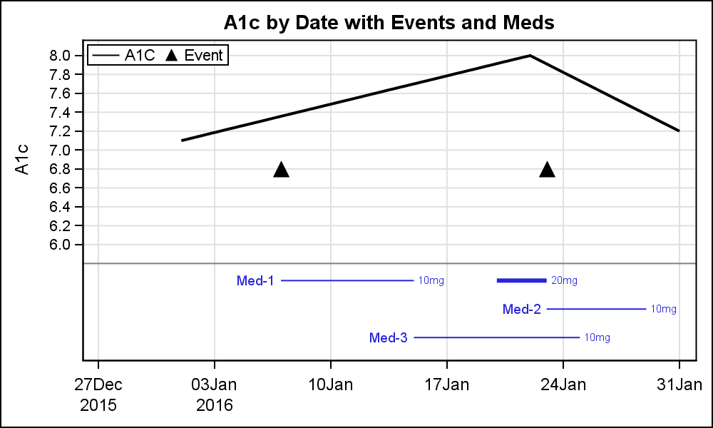A 2-cell SG plot is shown on the right.  Note the lack of a "row gutter" between the upper and lower sections, as these are all part of one cell.

See Full code:  A1C_Plot