Authors: Shahrzad Azizzadeh, Pelin Cay, Shelly Hunt, and Rob Wetzel

Ensuring food safety in meat processing facilities requires systematic inspection coverage across all plants. However, managing inspector assignments presents significant operational challenges. These include determining the optimal workforce size, assigning specific facilities to qualified personnel, and scheduling daily routes to minimize travel costs while maximizing productivity. The challenge here is optimizing inspector assignments. This post walks through how we formulated this challenge as a Mixed Integer Linear Programming (MILP) problem. Then we solved it by using the SAS Optimization CAS Action Set in SAS Viya, with preprocessing and visualization handled by the SAS DATA step and PROC SGPLOT. You will learn how this approach can determine the minimum workforce size, optimize the inspector-type composition to reduce salary costs, and generate executable daily schedules with travel-feasible routes.

Operational challenge

Scheduling is often inefficient in this environment due to the sheer number of possible combinations. Schedulers must simultaneously account for disjointed geographic locations, varying inspector radius constraints, disparate certification levels (state vs. federal), and strict time windows. As the network grows, ensuring 100% coverage and accurately forecasting costs becomes computationally intractable without advanced optimization techniques.

Background

In this case study, we analyzed a state network comprising over 100 federal and state-licensed meat processing facilities. A major component of these facilities is federal establishments. To meet regulatory food safety requirements, these facilities require mandatory daily visits by licensed inspectors.  The current workforce consists of federal and state inspectors.

• Federal inspectors: Certified to inspect all federal facilities and may inspect state facilities under specific agreements.
• State inspectors: Authorized for state-licensed plants. The Talmadge-Aiken (TA) cooperative agreement also authorizes trained state inspectors to inspect federal facilities.

The Optimization Trade-Off

This certification hierarchy introduces a key economic lever. Federal inspectors typically command higher annual salaries than their state counterparts. Therefore, minimizing total operational costs often aligns with maximizing the utilization of state inspectors (via the TA program) wherever they are geographically and professionally eligible. However, strict adherence to certification constraints is required to ensure regulatory compliance.

Operationally, we estimate that each inspection takes an average of 1 hour. The inspection window runs from 8:00 AM to 8:00 PM. Unlike static assignment models, this project incorporates travel time as a decision variable. We treat the problem as a routing-and-scheduling optimization to maximize inspector productivity.

Use Case: Defining the Optimization Questions

This project utilizes SAS Optimization to answer three critical resource allocation questions:

Question 1: What is the minimum resource requirement?

Before assigning specific names to locations, we must determine the theoretical floor for the workforce size. How many inspectors are strictly necessary to cover the plant network's geographic spread during the operational window?

Question 2: What is the minimum-cost inspection workforce composition?

Once the headcount is established, we must optimize the mix of Federal vs. State inspectors. This involves identifying the ideal workforce structure that achieves 100% coverage while adhering to TA eligibility rules, aiming to minimize total salary overhead and travel expenses.

Question 3: What is the optimal daily schedule?

Finally, we must generate executable daily rosters. This requires assigning specific inspectors to specific facilities in precise time slots, ensuring that travel between sequential locations is feasible and minimized.

Input Data

The optimization system relies on several key data sources that define the problem structure. You can see the input data model in Table 1.

Data preprocessing

Before optimization can take place, several preprocessing steps are performed to structure the raw operational data into a format suitable for mathematical modeling. There are two key components of preprocessing. The first is creating time slots that define the available inspection periods for each day. The second is the generation of feasible transitions, which determine how inspectors can feasibly move between facilities over consecutive slots.

Scalability Note: The logic used here relies on standard geographic coordinates and time-window parameters, making this framework agnostic to specific state geographies. It is designed to be reusable and easily scalable to other states or regions with minimal configuration changes.

How time slots are created

Time slots define the basic scheduling framework for assigning inspectors to facilities. We generate these slots based on several things. One is the daily operating window. The other is the duration of each inspection, incorporating buffer times (time for inspector check-in and preparation) to ensure travel feasibility between consecutive assignments.

The daily inspection window spans from 8:00 AM to 8:00 PM, totaling 720 operational minutes. Based on the customer's operational data, each inspection is assumed to take 1 hour on average, followed by a 45-minute buffer to account for check-in, preparation, and transition time. Importantly, both the inspection duration and buffer time are configurable input parameters in the model. This enables agencies to adjust them based on their own operational experience. Using these parameters, the model divides the day into seven discrete time slots, each starting 105 minutes apart (60-minute inspection + 45-minute buffer). The buffer applies only between consecutive slots — not before the first slot or after the last. The final slot ends at 7:30 PM, leaving 30 minutes of slack before the window closes.

Not every inspector fills all seven slots. The model typically assigns three to five inspections per inspector per day, consistent with the observed baseline. The unused slots provide flexibility for travel between geographically dispersed facilities. This is handled by the feasible transitions logic described below.

How feasible transitions are created

To formulate the mathematical optimization model, we first define a set of feasible transitions. This would be the allowed consecutive assignments in which an inspector moves directly from one facility to the next in adjacent time slots.

In order to do this, we form a plants-slots set, then flag any (plant_from, slot_from) and (plant_to, slot_to) pairs where travel time (computed using travel speed of 35 MPH) exceeds available time (“start of slot_to” minus “end of slot_from+ buffer time”), as infeasible. Next, we start with a set containing all possible (inspector, plant, slot) combinations where adjacent slot pairs are joined to create potential back-to-back transitions.

Then we ensure the same inspector is eligible for both plants in both slots. Ineligible combinations are removed. Then any transition that was previously flagged as infeasible due to travel time is also excluded. Each row in the resulting table represents a feasible back-to-back arc (inspector, (from_plant, slot_from), (to_plant, slot_to)) to be assessed for daily schedules.

Mathematical Model

The optimization problem is formulated as a Mixed Integer Linear Programming (MILP) model. The main components of the model include:

Decision Variables

• Assignment Variables: Binary variables indicating whether a certain inspector is assigned to a certain plant during a certain time slot. These form the core assignment decisions and are only defined over feasible (inspector, plant, slot) combinations.
• Inspector Utilization Variables: Binary variables indicating whether a certain inspector is selected for use in the overall solution.
• Travel Arc Variables: Binary variables capturing consecutive assignments — that is, whether a given inspector travels directly from one facility to the next in adjacent time slots (for example, Plant A in slot 1 followed by Plant B in slot 2).

Objective Function

The objective is to minimize the total annual cost, comprising two components:

• Annual Inspector Salaries: Sum of annual salaries for all selected inspectors.

Annualized Travel Costs

The daily travel cost associated with each consecutive facility-to-facility movement is multiplied by a per-mile cost rate and annualized over 365 operating days. Each inspector's first trip of the day — from their home location to their first assigned facility — is accounted for separately by using the inspector-to-plant distance data (the DISTANCES table). The model assumes a consistent daily schedule; in practice, variations such as weekend coverage or PTO can be incorporated by running the model under multiple scenarios or adjusting the annualization factor.

Constraints

• Coverage Requirements: Ensuring that each plant receives exactly one inspection visit per day.
• Inspector Capacity: Each inspector can be assigned to at most one plant during any given time slot.
• Inspector Eligibility: Only qualified inspectors can be assigned to a particular plant.
• Travel Feasibility: Consecutive assignments for an inspector to two plants that are too far apart are not accepted.

Results

The model was implemented and solved in SAS Viya 4.0 by using the SAS Optimization CAS Action Set, accompanied by extensive preprocessing and postprocessing steps implemented primarily in SAS DATA steps. For Visualizations, SAS PROC SGPLOT was used.

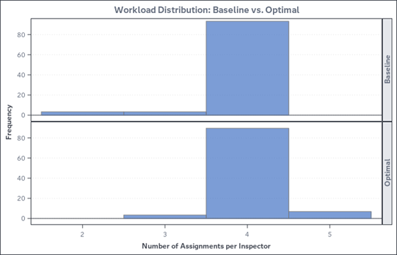
Optimal results are compared with the baseline solution (the customer-provided status quo) in Table 2. The model achieved significant efficiency gains. In the baselineleaving substantial idle capacity. The optimized solution consolidates assignments so that more inspectors handle four or five facilities per day along travel-efficient routes, reducing the total number of inspectors needed while increasing individual utilization (see Figure 1).

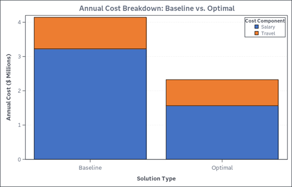
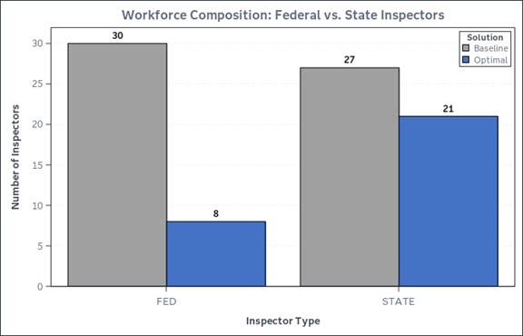
The workload distribution is presented in Figure 1. Cost breakdown and workforce composition are shown in Figures 2 and 3, respectively. You can see in Figure 3 that the optimal solution shifts the workforce mix toward more state inspectors operating under the Talmadge-Aiken (TA) Act. This leverages their lower cost while maintaining full plant coverage.

Conclusion

This project demonstrates how advanced analytics can transform a complex scheduling challenge into a clear, data-driven strategy. By implementing a mathematical model in SAS Optimization that accounts for inspector eligibility, travel constraints, and mandatory daily coverage, we successfully generated inspection schedules that are operationally feasible and highly cost-efficient.

Key Findings

Under our most aggressive optimization scenarios, the model indicates that in a sample state, the entire facility network -- 117 federal and state meat processing plants -- could be covered by a streamlined state workforce alone. By maximizing cross-utilization under the Talmadge-Aiken program, the model’s most aggressive assignment case shows a pathway to complete coverage with 30% fewer state personnel, while theoretically eliminating the need for deployed federal inspectors (a 100% reduction). More realistically, even after accounting for PTO and maintaining a reasonable workforce buffer, coverage could still be achieved by using only state resources. Overall, this result shows the benefits of an automated scheduling system based on employee radius, plant location, and optimizing route and driving distance. Today, assignments are often scheduled manually. Furthermore, if the Talmadge-Aiken program were expanded, the federal government could project costs and reimburse states in advance, rather than paying in arrears, creating funding issues.

Impact & Scalability

Beyond immediate cost savings, we have established a repeatable, scalable framework. Because the underlying code utilizes standardized input parameters (geographic coordinates, time windows, and eligibility matrices), this model is agnostic to specific state geographies and can be rapidly deployed to other inspection agencies. It serves not merely as a one-time fix but as a robust planning tool, empowering decision-makers to continuously explore "what-if" scenarios regarding budget adjustments, new plant openings, or policy changes with mathematical precision.

Pelin Cay
Pelin Cay has been with SAS since 2016 and is a Manager in the Applied AI & Modeling division. She leads a team of data scientists specializing in the design of advanced mathematical optimization models and solution methodologies for complex decision-making problems across diverse industries. Pelin earned her B.S. and M.S. in Industrial Engineering from Bilkent University and her Ph.D. in Industrial Engineering from Lehigh University.

Shelly Hunt
Shelly Hunt is a Systems Engineer at SAS, supporting USDA and FDA programs with advanced agriculture analytics and environmental modeling. She specializes in translating complex agricultural domain expertise into data science parameters that drive optimization models and large‑scale analytic workflows. Shelly holds a Master of Science in Biological and Agricultural Engineering and a Graduate Certificate in Agricultural Data Science, both from NC State University.

Rob Wetzel
Rob Wetzel is a Sr. Account Executive at SAS.