SAS® Fast-KPCA: An efficient and innovative nonlinear principal components method

Kernel Principal Components Analysis (KPCA) is an extension of PCA, which performs nonlinear dimension reduction. This is especially useful when we need to separate clusters that are not convex(not spherical or not elliptical). One advantage of KPCA versus PCA is that it is not bounded by the number of features/variables p but by the number of rows/observations n. It works by increasing the dimension of the space so that the resulting observations at the higher dimensional space can be separated and classified.

The exact implementation of KPCA utilizes the singular value decomposition (SVD) on the full inner product space, which is n by n. On larger data sets, running the exact method can be prohibitive or impossible to complete in a reasonable time. Additionally, for most input data sets, a smaller number of dimensions can explain most of the variation. SAS® Fast-KPCA implementation bypasses the limitations of the exact method by approximating the SVD using the Nyström method (Halko, 2009).

Before computing the SVD, existing implementations randomly sample the input data set to include only c observations to improve efficiency. SAS has implemented both an exact and Fast-KPCA. Fast-KPCA also subsets the input data to c components. Instead of randomly sampling to reduce the number of observations before computing the SVD, SAS selects c representative points by performing k-means on the original n observations. Using k-means to find the representative sample has the advantage that the c centroids are chosen to minimize the variation of points nearest to each centroid and maximize the variation to the other centroids. In some cases, the downstream effect of using k-means on computing the SVD increases numerical stability and improves clustering, discrimination, and classification.

In the following example, we use simulated data on the performance of a centrifugal pump that moves water from a tank upward to a set of pipes in a factory. The data simulated on the centrifugal pump is the pump head which is the height at which water can be lifted in a column against gravity, and the discharge flow rate, which is the volume of water that the pump can clear in an hour. There is a non-linear inverse relationship between the pump head and flow rate. The data has two clusters, one for normal operations and one for faults where the stationary wear ring on the impeller is blocking the clearance of liquid being removed by the pump.

The following DATA step simulates the data and plots the relationship between flow rate and pump head.

cas; 
caslib _all_ assign;
 
data casuser.centrifugal_pump;
   length Pump_Head 8 Flow_Rate 8 group $ 48;
   format Pump_Head Flow_Rate best12. group $char48.;
   label flow_rate= "Flow Rate at the Pump Outlet (meters^3/hour)"
         Pump_Head= "Pump Head (meters)";
   /*Normal Operations*/
   do i=1 to 10000;
      if i le 9500 then do;
         group="Normal Wear Ring Clearance";
         flow_rate = rand("Uniform", 7, 42);;
         Pump_Head = 67 - 0.0368*(flow_rate*flow_rate) + rand("Normal", 0, 0.25);
         output;
      end;
      else do;
         group="Low Wear Ring Clearance";
         flow_rate = rand("Uniform", 7, 42);;
         Pump_Head = 74 - 0.0361*(flow_rate*flow_rate) + rand("Normal", 0, 0.65);
         output;
      end; 
   end;
run;
 
ods graphics;
proc sgplot data=casuser.centrifugal_pump;
   scatter x=flow_rate y=Pump_Head / group=group;
run;

In the following graph, the faults are colored in blue and normal operations are in gold. Our objective is to separate the two groups so we can model the normal and the fault group dynamics separately and discriminate faults in a streaming fashion during pump operation.

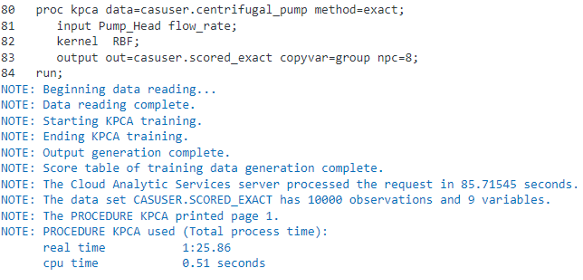
If we run the exact method,

proc kpca data=casuser.centrifugal_pump method=exact;
   input Pump_Head flow_rate;
   kernel  RBF;
   output out=casuser.scored_exact copyvar=group npc=8;
run;

the total elapsed time to run our example is approximately 1 minute and 25 seconds.

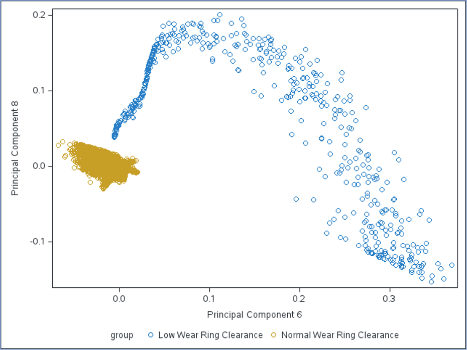
If we plot the 6th and 8th principal components, we can see that the faults can be linearly separated from normal observations:

PROC DISCRIM will be used to run a linear discriminant analysis to split the two groups using the scored principal components from the exact method.

proc discrim data=casuser.scored_exact method=normal pool=yes short;
  class group;
  priors proportional;
run;

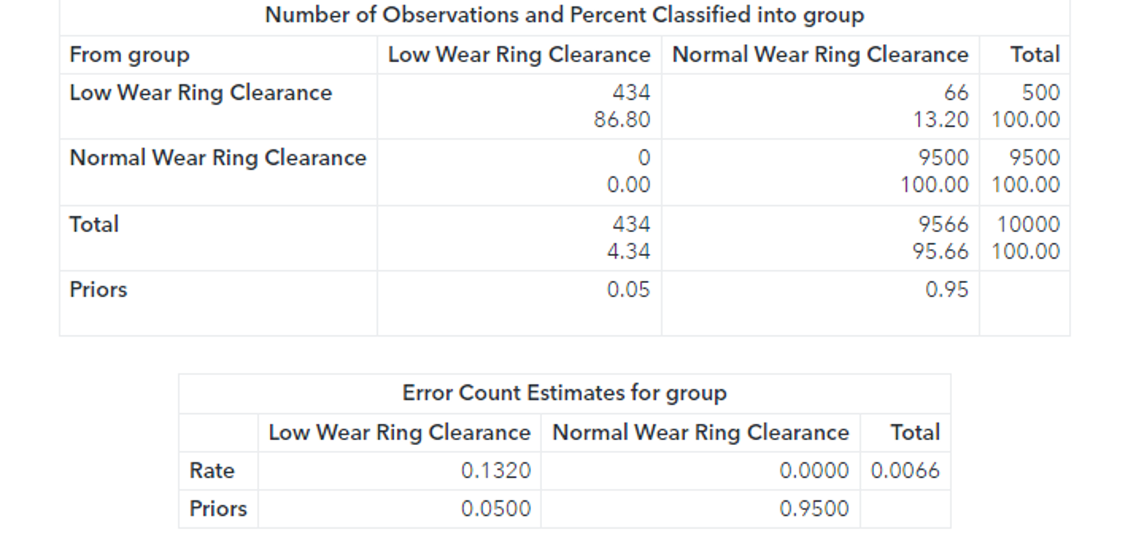
The confusion matrix shows that 66 faults were classified as normal observations. The total misclassification rate for this sample is 0.0066 or 0.66%.

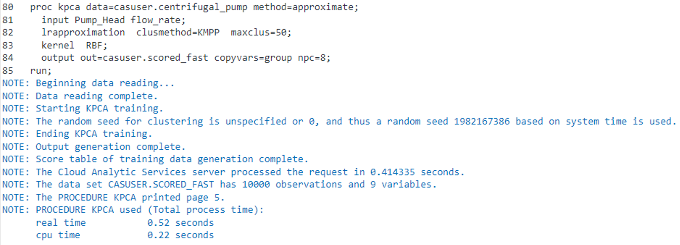
We will run the Fast-KPCA method by specifying METHOD=APPROXIMATE on the KPCA statement. Additionally, we will specify the use of k-means to reduce the observations by specifying CLUSMETHOD=KMPP on the LRAPPROXIMATION statement.

proc kpca data=casuser.centrifugal_pump method=approximate;
   input Pump_Head flow_rate;
   lrapproximation clusmethod=kmpp maxclus=50;
   kernel  RBF;
   output out=casuser.scored_fast copyvar=group npc=8;
run;

Using the Fast-KPCA method, we can see that the total elapsed time has reduced considerably to approximately .5 seconds, which is a considerable improvement over the exact method.

Additionally, while the Fast-KPCA method is extremely efficient, the accuracy of the linear discriminant is the same as the exact method. The confusion matrix shows that 66 faults were classified as normal observations. The total misclassification rate for this sample is 0.0066 or 0.66%. 66 observations out of 10000 observations were misclassified.

proc discrim data=casuser.scored_fast method=normal pool=yes short;
  class group;
  priors proportional;
run;

References

SAS® Viya® Programming Documentation, Data Mining and Machine Learning Procedures, The KPCA Procedure, https://go.documentation.sas.com/doc/en/pgmsascdc/v_032/casml/casml_kpca_example01.htm,

Halko, N. and Martinsson, P. G. and Tropp, J. A. (2009) Finding Structure with Randomness: Stochastic Algorithms for Constructing Approximate Matrix Decompositions. ACM Technical Reports, 2009-05.

M. Li, W. Bi, J. T. Kwok, and B. -L. Lu, "Large-Scale Nyström Kernel Matrix Approximation Using Randomized SVD," in IEEE Transactions on Neural Networks and Learning Systems, vol. 26, no. 1, pp. 152-164, Jan. 2015.