Building a large high-quality corpus for Natural Language Processing (NLP) is not for the faint of heart. Text data can be large, cumbersome, and unwieldy and unlike clean numbers or categorical data in rows and columns, discerning differences between documents can be challenging. In organizations where documents are shared, modified, and shared again before being saved in an archive, the problem of duplication can become overwhelming.

To find exact duplicates, matching all string pairs is the simplest approach, but it is not a very efficient or sufficient technique. Using the MD5 or SHA-1 hash algorithms can get us a correct outcome with a faster speed, yet near-duplicates would still not be on the radar. Text similarity is useful for finding files that look alike. There are various approaches to this and each of them has its own way to define documents that are considered duplicates. Furthermore, the definition of duplicate documents has implications for the type of processing and the results produced. Below are some of the options.

Using SAS Visual Text Analytics, you can customize and accomplish this task during your corpus analysis journey either with Python SWAT package or with PROC SQL in SAS.

Work with Python SWAT

The Python SWAT package provides us with a Python interface to SAS Cloud Analytic Services (CAS). In this article, we’ll call the profileText action, pull down output tables, and perform duplicate identification in Python.

Prepare the data

The corpus we’re going to explore is Second Release of the American National Corpus (ANC2). It’s also one of the reference corpora for the profileText action. The corpus contains over 22,000,000 words of written and spoken texts and comes with both annotated data and their plain texts.

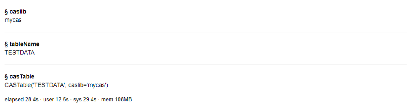
We put all 13295 plain text files under /home/anc2. After connecting to the CAS server, we create the table TESTDATA with ANC2 data.

# Import libraries
import swat
from collections import Counter
import pandas as pd
import itertools
import random
 
# Connect to CAS server
s = swat.CAS("cloud.example.com", 5570)
 
# Add the caslib mycas with the path to corpus directory
s.addCaslib(caslib='mycas',
            datasource={"srcType":"path"},
            session=False,
            path="/home",
            subdirectories="yes")
 
# Load txt files under anc/ to the CASTable testdata
s.loadTable(casout={"name":"TESTDATA", "replace":True},
            caslib="mycas",
            importOptions={"fileType":"Document"},
            path="anc2")

Out:

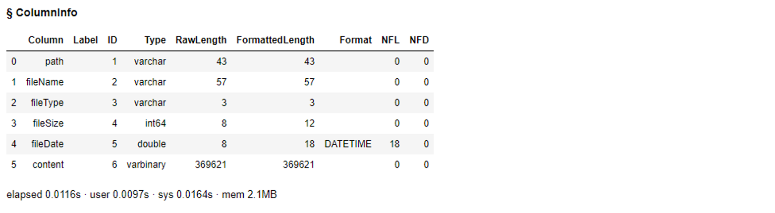
We can check on the table easily, such as by using columnInfo() or head().

# View column summary for testdata
anc2 = s.CASTable("TESTDATA", replace=True)
anc2.columninfo()

Out:

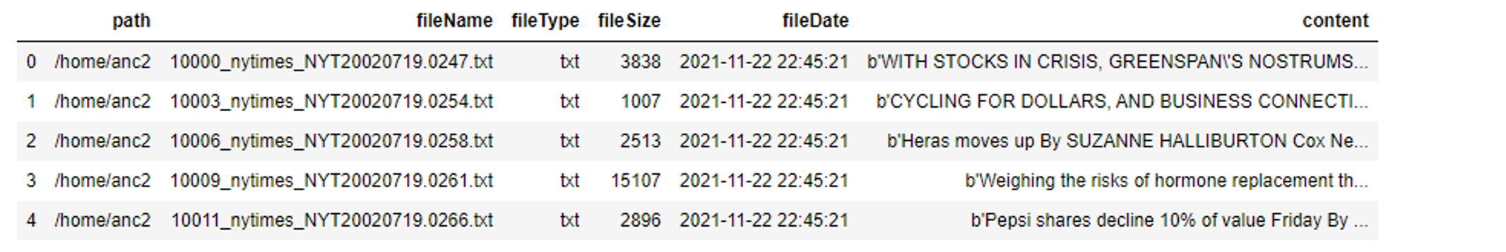
# Check on the first five rows
anc2.head()

Out:

Profile the data

We load the Text Management action set and call the profileText action to profile the ANC2 data. The casOut parameter is required to run the action. This output table contains information complexity, information density, and vocabulary diversity statistics. For duplicate identification we need the results from two output tables, documentOut and intermediateOut. A CASTable can be converted to a SASDataFrame by using the CASTable.to_frame() method. This method helps us pull all of the data down for further exploration.

# Load the action set textManagement
s.loadactionset('textManagement')
 
# Call the action profileText
results = s.profileText(table=dict(caslib="mycas", name="testdata"),
                        documentid="fileName",
                        text="content",
                        language="english",
                        casOut=dict(name="casOut", replace=True),
                        documentOut=dict(name="docOut", replace=True),
                        intermediateOut=dict(name="interOut", replace=True))

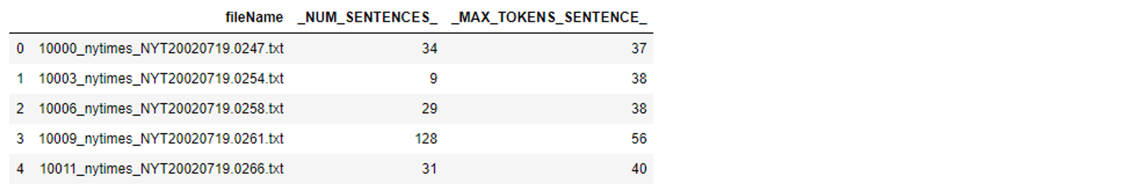
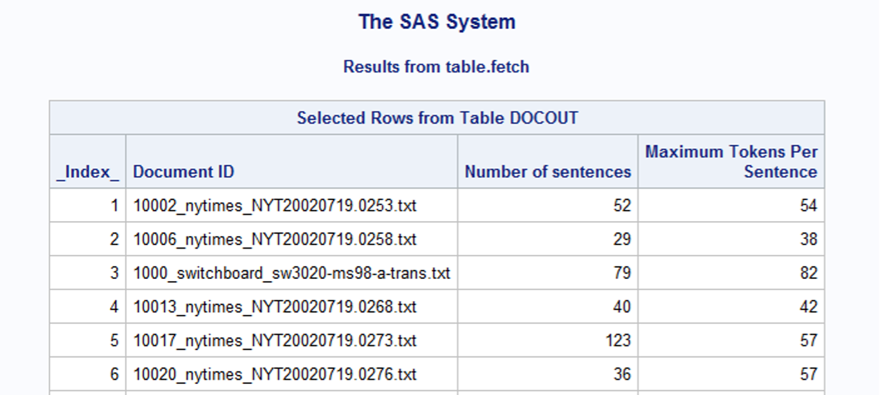
The documentOut contains document-level information complexity statistics. For each file, we know their total number of sentences and maximum number of tokens in these sentences.

# Convert the CASTable docOut to SASDataFrame
df_docout = s.CASTable('docOut').to_frame()
df_docout.head()

Out:

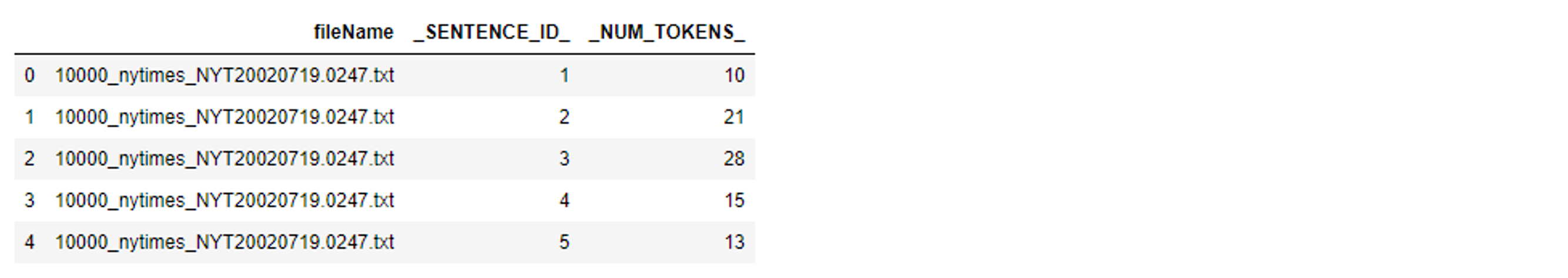
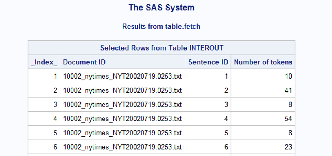
The other output, intermediateOut, contains the token count of each sentence in each document.

# Convert the CASTable interOut to SASDataFrame
df_interout = s.CASTable('interOut').to_frame()
df_interout.head()

Out:

Filter the data

Our goal is to locate both identical documents and documents that are not identical but substantially similar. To narrow our search results for good candidates, we introduce an assumption that if two files have the same number of sentences and the maximum number of tokens for a sentence, they have a higher possibility to be duplicates or near-duplicates.

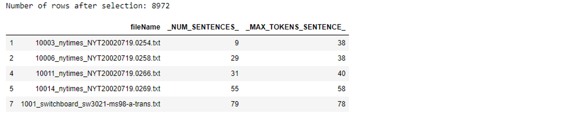
Having this assumption, we keep the documents with their value pair of _NUM_SENTENCES_ and _MAX_TOKENS_SENTENCES_ occurring more than once, leaving us 8972 out of 13295 files.

# Filter out docs with their column values appearing more than once
df_docout_selected = df_docout[df_docout.groupby(['_NUM_SENTENCES_','_MAX_TOKENS_SENTENCE_'])
                                                 ['_NUM_SENTENCES_'].transform('size')>1]
print(f"Number of rows after selection: {len(df_docout_selected)}")
df_docout_selected.head()

Out:

You can further reduce results if there’s a focus in your search by providing conditions like, only selecting documents with a total number of sentences of more than 200, or selecting those with a maximum number of tokens in a sentence of more than 80.

# (Optional) Reduce search results by filtering out docs by condition
df_docout_selected=df_docout_selected[df_docout_selected._NUM_SENTENCES_>200]
df_docout_selected=df_docout_selected[df_docout_selected._MAX_TOKENS_SENTENCE_>80]

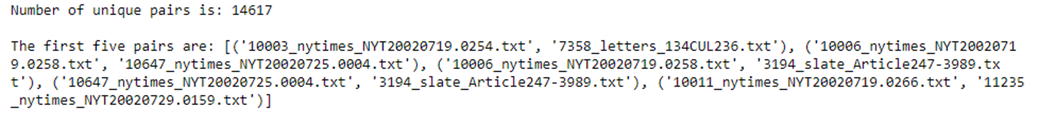
Next, we prepare pair combinations of files that share the values for _NUM_SENTENCES_ and _MAX_TOKENS_SENTENCES_. Notice that sometimes more than 2 files share the same values. The total number of unique pairs is 14617.

# Keep only the interout data for files that are selected
search_dict = df_docout_selected.set_index('fileName').T.to_dict('list')
df_interout_selected = df_interout[df_interout['fileName'].isin(search_dict.keys())]
 
# Get all unique combinations of every two docs
check_tmp_dict = Counter([tuple(s) for s in search_dict.values()])
file_pair_lst = []
for c in check_tmp_dict:
    file_pair = [k for k,v in search_dict.items() if tuple(v)==c]
    if len(file_pair) == 2:
        file_pair_lst.append(tuple(file_pair))
    else:
        pair_lst = list(itertools.combinations(file_pair, 2))
        file_pair_lst += pair_lst
 
print(f"Number of unique pairs is: {len(file_pair_lst)}\n")
print(f"The first five pairs are: {file_pair_lst[:5]}")

Out:

Compare the data

Finding textual near duplicates is more complicated than duplicates. There is no gold standard on the similarity threshold of two considered near-duplicates. Based on the _NUM_TOKENS_ by _SENTENCE_ID_ from the table interOut earlier, we add the assumption that two documents have a very high possibility to be near-duplicates if they share the same number of tokens for the sentences ordered in a list with their indices randomly picked by a defined ratio to total sentence number.

For example, fileA and fileB have 20 sentences each and the defined ratio is 0.5. We use pandas.Series.sample to randomly select 10 sentences from two files each. The random_state value is required to make sure that sentences from two files are picked up in parallel. If the two sentences have the same number of tokens for every pair we sampled, fileA and fileB are considered near-duplicates.

Now we are ready for comparison.

# Compare doc pairs
possibleDuplicate = []
for (a, b) in file_pair_lst:
    # Keep only the column _NUM_TOKENS_
    tmp_a = df_interout_selected[df_interout_selected['fileName']==a].loc[:,"_NUM_TOKENS_"]
    tmp_b = df_interout_selected[df_interout_selected['fileName']==b].loc[:,"_NUM_TOKENS_"]
    # Drop the index column to use pandas.Series.compare
    tmp_a.reset_index(drop=True, inplace=True)
    tmp_b.reset_index(drop=True, inplace=True)
    # Select sentences by pandas.Series.sample with the defined ratio
    num_sent, num_sent_tocheck = len(tmp_a), round(ratio_tocheck*len(tmp_a))
    tmp_a = tmp_a.sample(num_sent_tocheck, random_state=1)
    tmp_b = tmp_b.sample(num_sent_tocheck, random_state=1)
    # Detect duplicates by checking whether it is an empty dataframe (with a shape of (0,2))
    if tmp_a.compare(tmp_b).shape != (0,2):
        pass
    else:
        possibleDuplicate.append([a, b])

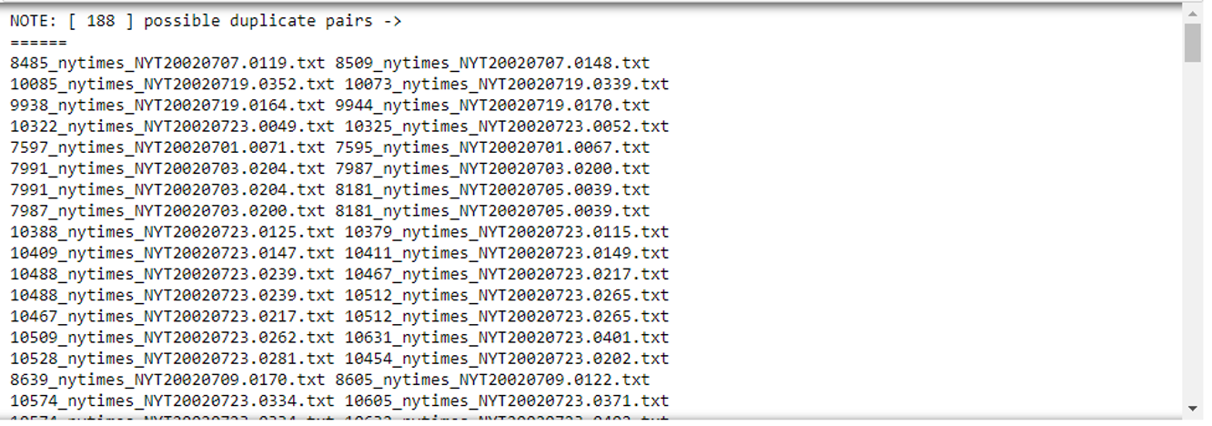
The possibleDuplicate list contains 188 pairs of file names.

# View the result
view = '======\n'+'\n'.join([" ".join(p) for p in possibleDuplicate])+'\n======'
print(f"NOTE: [ {len(possibleDuplicate) } ] possible duplicate pairs -> \n{view}")

Out:

Verify the results

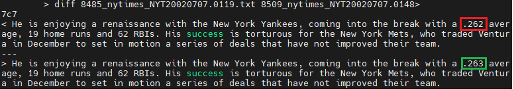
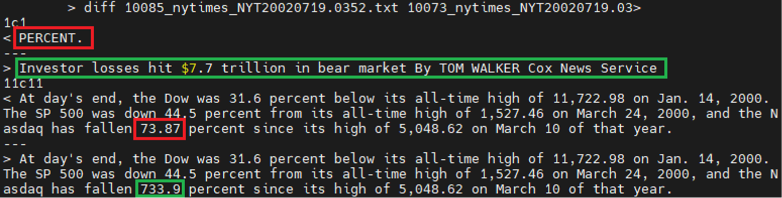
Now it’s time to see how far we went for our duplicate search. By checking the content of each pair, it’s not hard to find 133 being duplicates and 55 being near duplicates. Let’s take a look at two near-duplicate pairs we find. These documents have around 50 sentences and the differences occur just between 2 sentences.

Work with PROC SQL in SAS

SQL is one of the many languages built into the SAS system. Using PROC SQL, you have access to a robust data manipulation and query tool.

Prepare the data

We load the folder /home/anc2 with all plain text files to the table TESTDATA.

libname mycas cas;
 
proc cas;
  table.addcaslib /
    caslib = "mycas"
    datasource = {srctype="path"}
    session = False
    path = "/home"
    subdirectories = "yes";
run;
 
  table.loadTable /
    casout = {name="testdata", replace=True}
    caslib = "mycas"
    importOptions = {fileType="DOCUMENT"}
    path = "anc2";
run;
quit;

You can load it directly if you have already saved them to a .sashdata file.

proc cas;
  table.save /
    table = {name="testdata"}
    caslib = "mycas"
    name = "ANC2.sashdat";
run;
 
  table.loadtable /
    casout = {name="testdata", replace=true}
    path = "ANC2.sashdat"
    caslib = "mycas";
run;
quit;

Profile the data

We call the profileText action in the textManagement action set to profile the data.

proc cas;
  textManagement.profiletext /
    table = {name="testdata"}
    documentid = "fileName"
    text = "content"
    language = "english"
    casOut = {name="casOut", replace=True}
    documentOut = {name="docOut", replace=True}
    intermediateOut = {name="interOut", replace=True};
  run;
 
  table.fetch /
    table = {name="docOut"};
  run;
 
  table.fetch /
    table = {name="interOut"};
  run;
quit;

Filter the data

We keep the documents given that their value pair occurs more than once.

proc sql;
  create table search1 as
    select * from mycas.docout
    group by _NUM_SENTENCES_, _MAX_TOKENS_SENTENCE_
    having count(*) > 1;
quit;

We prepare all pair combinations of files that share the same values.

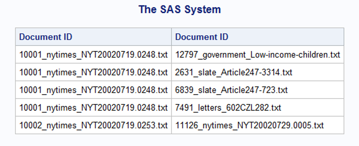
proc sql;
  create table search2 as
    select a.fileName as fileA , b.fileName as fileB
    from
      (select * from search1 ) a
        cross join
      (select * from search1 ) b
    where a._NUM_SENTENCES_ = b._NUM_SENTENCES_ and
      a._MAX_TOKENS_SENTENCE_ = b._MAX_TOKENS_SENTENCE_ and
      a.fileName <> b.fileName;
quit;
 
proc print data=search2(obs=5);
run;

With a glimpse of table search2, we notice that it would be better to get just unique pairs to avoid repeating comparing those with the same file names.

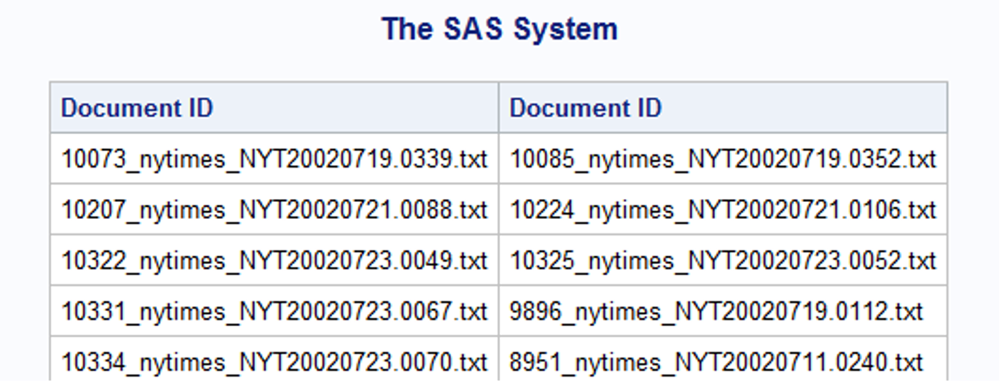
proc sql;
  create table search3 as
    select distinct fileA, fileB from search2
    where search2.fileA < search2.fileB;
quit;
 
proc print data=search3(obs=5);
run;

Compare the data

Given the assumption that two documents have a very high possibility to be near-duplicates if they share the same number of tokens for the sentences ordered in a list with their indices randomly picked by a defined ratio to total sentence number. Here we use the rand(‘uniform’) function to generate an observation from the continuous uniform distribution in the interval (0,1) as default. Setting it with ‘between .2 and .7’ helps us randomly get 50% of sentences. The similarity threshold can be customized by changing the range, say “where rand(‘uniform’) between .2 and .9” which means 70% of sentences in the documents would be examined.

proc sql;
  create table search4 as
    select fileA as f1, fileB as f2 from search3 
    where not exists (
      select * from (
        select tmp1A, tmp2A from (
          select tmp1._NUM_TOKENS_ as tmp1A, tmp1._SENTENCE_ID_ as tmp1B,
                 tmp2._NUM_TOKENS_ as tmp2A, tmp2._SENTENCE_ID_ as tmp2B from
            (select * from sasout1.interout interout1 where interout1.fileName = f1) tmp1,
            (select * from sasout1.interout interout2 where interout2.fileName = f2) tmp2 
	    where tmp1B = tmp2B)
          where rand('uniform') between .2 and .7)
        where tmp1A <> tmp2A);
quit;

Verify the results

We use the table testdata to verify the results. There are 133 duplicates and 39 near duplicates out of 172 pairs.

proc sql;
  create table Duplicates as
    select f1, f2 from search4
    where not exists (
      (select content from mycas.testdata tmp where tmp.fileName = f1)
      except
      (select content from mycas.testdata tmp where tmp.fileName = f2)
    );
quit;
 
proc sql;
  create table nearDuplicates as
    select f1, f2 from search4
    where exists (
      (select content from mycas.testdata tmp where tmp.fileName = f1)
      except
      (select content from mycas.testdata tmp where tmp.fileName = f2)
    );
quit;

Conclusions

Exploring derived statistics from the profileText action provides a practical perspective to gain insights not only by comparing to a reference corpus, but at token, sentence, and document levels within a corpus itself. With the randomness in selecting which sentences to compare, we might observe different results after performing this duplication identification method. The smaller ratio we define, the more near-duplicate pairs we get. And you would probably be surprised by the fact that if we set the ratio to 0.1, the result would still be around 207 pairs, just a little bit more than 172 pairs when the ratio is set to 0.5. The method doesn’t seem to overfire because two files are required to have the same number of sentences and the same maximum number of tokens in a sentence before we pair them up. This requirement gives us a safer place to start our search.

Textual near duplicate identification is simple to understand but not easy to develop standards to include every type of near duplicates. In this article, we provide one way to describe near duplicates in which distance is between several sentences or words in order, yet not including cases like sentences of two documents are not arranged in the same order or some chunks are glued together so that the results are affected by different sentence indexing. These are fun to think about and they might be turned into the next level detection.

How would you define the similarity for near duplicates?

Learn more

• Check out additional documentation on corpus analysis and  SAS Visual Text Analytics.
• Keep exploring by checking out the ebook “Make Every Voice Heard with Natural Language Processing” or visit SAS Visual Text Analytics.