This post will describe how to generate heat maps in CAS by using the DATA step action to calculate 2D histograms and the Image action set for postprocessing. The algorithm in this example is a practical application of one of the use cases presented in a previous post. In that post, we proposed using heat maps as one way to anonymize people being viewed by a security camera.

Extending beyond privacy protection, this example not only uses heat maps as an anonymization tool but also uses them to draw inferences about how an environment is utilized. Specifically, we are identifying heavily trafficked zones. The complete source code is available on GitHub.

Overview of the image processing pipeline

For this application, the motion tracking data was collected separately from the heat map calculations. The heat maps accumulated tracking data across a user-specified time window, five minutes for example, and at a user-specified resolution. The processing pipeline for the heat map calculations was:

1. Load the motion tracking data and base image
2. Preprocessing:
   • Convert tracked object bounding box coordinates to a centroid coordinate
   • Filter the centroids that are out of the image boundary
   • Group the tracked object coordinates by time window
3. 2D histogram calculation with resolution NxN
4. Postprocessing:
   • Transform the histogram data to an NxNx1 dimension image
   • Normalize and rescale the histogram bin values to 8-bit integers
   • Resize the NxNx1 image to the height and width of the base image
5. Overlay the heat map on the base image

The pipeline can be visualized below:

Loading data details

The motion tracking data for this algorithm was stored in a CSV file. The file has columns for the frame number (embedded in an image file name) and the coordinates of the top-left and bottom-right corners of the tracked objects bounding box. The loadTable action will handle loading the CSV file for us.

We will also want to load the base image at this stage. The dimensions of the base image will be used in later processing to filter out tracked objects that leave the image boundary. We can use the loadImages action for this.

Check out the ‘Load Tracking Data and Base Image’ section of the Jupyter Notebook on GitHub to see how these two actions were used.

Preprocessing details

The preprocessing was accomplished using a call to the DATA Step action set. The preprocessing is primarily needed to assign a time window ID. This is determined by an interval specified by the user. It also assigns the frame rate in which images were captured. A few other simple preprocessing calculations are made in this first pass of the data. Namely, converting each object’s bounding box coordinates to a centroid coordinate and then filtering out any centroids that leave the image boundary.

   preprocessed_data = s.CASTable('preprocessed_data', replace=True)
   response = s.datastep.runcode(
       code=f'''data preprocessed_data;
                set tracking_data;
 
                /* Calculate centroids from the top-left and bottom-right bounding box coordinates. */
                cx = BRx/2 + TLx/2;
                cy = BRy/2 + TLy/2;
 
                /* Filter out any centroids that leave the image boundary. */
                if cx >= 0 and cx < {width} and cy >= 0 and cy < {height} then do;
 
                    /* Parse the frame number from the filename and then calculate the time window ID based on
                       the frame number, framerate, and window length (in minutes). */
                    time_window_id = floor((int(scan(filename,-2,'_./'))-1) / {heatmap_window_minutes*60*framerate});
 
                    output; 
                end;
             run;
   ''')

2D histogram calculation details

The DATA Step action set is again leveraged, but this time it’s used to calculate 2D histograms. There are several important nuances to point out with the histogram calculation:

1. We use the BY statement on the time window ID to ensure that each histogram corresponds to a specific window in time
2. The tracked objects are binned in the 2D histogram, where the histogram bins range from 0 to N-1
3. The 2D array type used in the DATA step will be automatically flattened into a wide table

The 2D histogram binning can be visualized in Figure 2. In this example, a 300x300 pixel image is transformed into a 3x3 2D histogram. The 3x3 2D histogram is ultimately flattened into a single row with nine columns. In the example, a tracked object is detected at pixel location (205, 95) and binned in row-1 column-3 of the 2D histogram (shown in light blue). After flattening, row-1 column-3 of the 2D histogram becomes column 3 in the output table, shown on the right.

The 2D histogram calculation illustrated in Figure 2 was implemented using the DATA step shown below.

   total_num_bins = heatmap_resolution*heatmap_resolution
   pixels_per_bin = width/heatmap_resolution
 
   histograms = s.CASTable('histograms', replace=True)
   response = s.datastep.runcode(
       code=f'''data histograms (keep=c01-c{total_num_bins} time_window_id);
                 set preprocessed_data;
 
                 /* Process by time_window_id to get one histogram per time interval.*/
                 by time_window_id;
 
                 /* Create histogram bins and instruct DATA step to retain values between rows.*/
                 array histogram_bins{{{heatmap_resolution},{heatmap_resolution}}} c01-c{total_num_bins};
                 retain histogram_bins;
 
                 /* 'Bin' the centroid coordinates.*/
                 x = floor(cx/{pixels_per_bin})+1;
                 y = floor(cy/{pixels_per_bin})+1;
 
                 /* Increment the histogram bin values based on the binned coordinates.*/
                 if histogram_bins{{y,x}}=. then histogram_bins{{y,x}}=1;
                 else histogram_bins{{y,x}}=histogram_bins{{y,x}}+1;
 
                 /* When all observations in a time window are processed, write the result to the output table.*/
                 if last.time_window_id then output;
             run;
   ''')

Postprocessing details

A key benefit to using the DATA step for the 2D histogram was that the histogram was transformed into a wide table for free during the calculations. This is significant because the Image action set has an action, condenseImages, that transforms a wide table into a single image column. This can then be used within the Image action set.

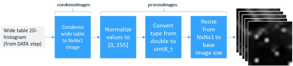
In the postprocessing, illustrated in Figure 3, we use the condenseImages action to transform a wide table into an image. Then the processImages action is used to prepare the histogram bin values for use as an image before finally resizing the histogram to fit our base image. For visualizing café-utilization we want a spatial heat map with continuously varying magnitude. To accomplish this the resizing step uses bilinear interpolation when transforming the NxNx1 image to the base image size.

The pipeline is shown below. The source code for this section is located in the postprocessing’ section of the Jupyter Notebook previously referenced.

Heat map overlay details

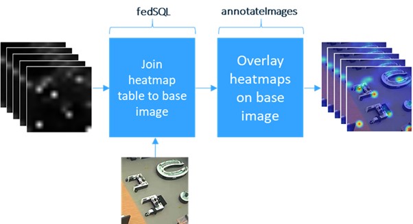
At this stage in the pipeline, we have a table with heat maps corresponding to each window in time the user specified. The annotateImages action, found in the Image action set, can be used to overlay these heat maps on the base image. However, the table of heat maps must be joined with the base image first. We use the fedSQL action set to perform the table-join. Check out the section ‘Overlay the Heat map on Base Image’ on GitHub to see the code for this step. The diagram in Figure 4 illustrates the overlay sequence.

Performance

Comparisons were made between a Python implementation (using OpenCV and NumPy for image processing and 2D-histogram calculations) and the CAS version described here. All tests were repeated five times, and the average run times were reported.

For the first test, comparisons were made by holding the 2D histogram resolution constant (at N=13) and varying the size of the heat map time window. In Figure 5 you see a comparison of the basic Python implementation and the CAS version running in both single-machine mode (SMP) and distributed mode (MPP). Figure 6 zooms in only on the CAS version.

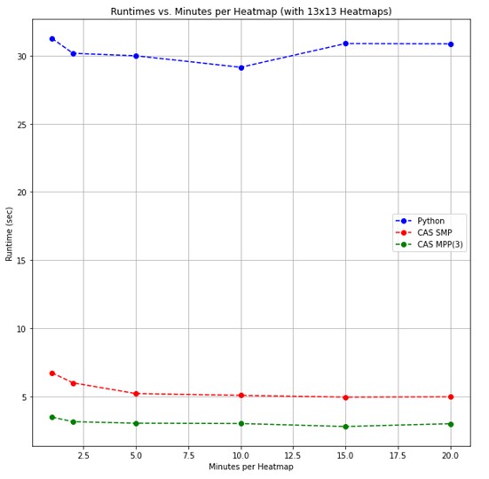
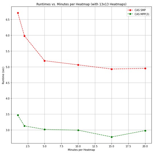
Looking at Figure 5, the algorithm runs approximately 5x faster in SMP CAS, and 10x faster in MPP CAS, than in the basic Python implementation. The Python version has a constant run time when varying the heat map time window length because it can leverage the assumption that all observations are in order and can be processed sequentially. The CAS implementation run times vary slightly due to nuances with BY-group processing. That is, when the heat map window length is reduced, there are more windows to be processed, and additional overhead is added.

For a second test, the heat map time window was held constant (at five minutes per heat map) and the resolution of the 2D histogram was swept.

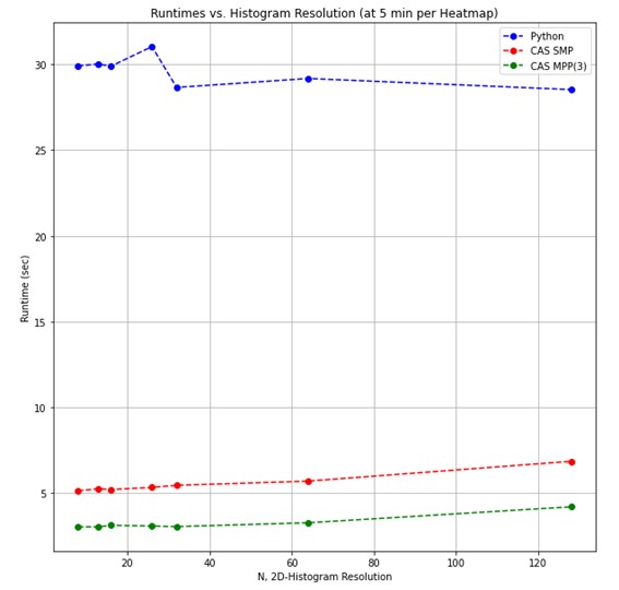
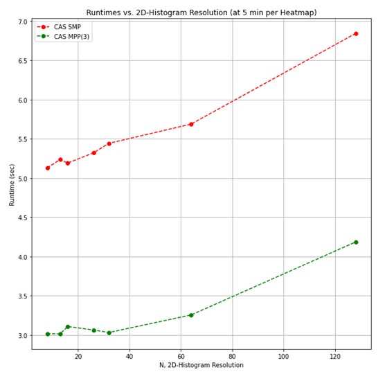
Again, the SMP CAS implementation is approximately 4-5x faster, and when in MPP about 8-10x faster. Just like in the first test, we see the Python version is near-constant in run time when we vary the histogram resolution. This time the constant run time is due to the 2D histogram calculation making use of efficient array data structures with O(1) access times. Conversely, the CAS implementation slightly increases with the resolution because the 2D histogram data is stored in a wide table where accesses are O(n).

Conclusion

Heat maps are a valuable tool whose uses range from simplifying data, like in the case of privacy-protected analytics discussed in a previous post, to the data visualization example which was highlighted in the café-utilization application here. While spatial heat maps were most useful to the café example, many other applications benefit from different types of heat maps, like grid heat maps, and can also be generated by changing the interpolation type in the resizing step of the postprocessing stage.

This heat map generation pipeline illustrates how the DATA Step action set can be used to extend the functionality of the Image action set. In this post, only the condenseImages action of the Image action set was used. But the flattenImages and condenseImages actions can be used together to move images out of and into image formats. This opens the door for any CAS action to be used on image data.