, you can have both")
In this post, I will provide an overview of generalized additive models (GAMs) and their desirable features. Predictive accuracy has long been an important goal of machine learning. But model interpretability has received more attention in recent years. Stakeholders, such as executives, regulators, and domain experts, often want to understand how and why a model makes its predictions before they trust it enough to use it in practice.
However, when you train a machine learning model, you typically face a tradeoff between accuracy and interpretability. GAMs provide a solution to this dilemma because they strike a nice balance between these two competing goals. With Model Studio, you can easily train GAMs alongside other common machine learning models to compare model performance, all without the need to write any code.
What are GAMs?
GAM is short for generalized additive model. Before we discuss GAMs, let’s first briefly review a common statistical model that you are likely to be familiar with. It is the generalized linear model (GLM). A GLM is a very popular and flexible extension of the classical linear regression model. It enables you to model a target (or response) variable that is not normally distributed.
For example, if you are interested in predicting whether an incoming email is spam, or you want to predict the number of people dining in a restaurant, the linear regression model is inappropriate. This is because the target variables for those applications violate the model’s normality assumption. However, a GLM can handle both data types by assuming a distribution in the exponential family and by using a link function to relate the linear predictor to the distribution mean. If you assume a Gaussian distribution and use an identity link function, then a GLM reverts to a classic linear regression.
A GAM, then, extends a GLM even further by relaxing the linearity assumption. For a target or response variable y, both GAMs and GLMs assume the additive model:
\(g(\mu_i)= f_1(x_{i1}) + f_2(x_{i2}) + \cdots + f_p(x_{ip})\)
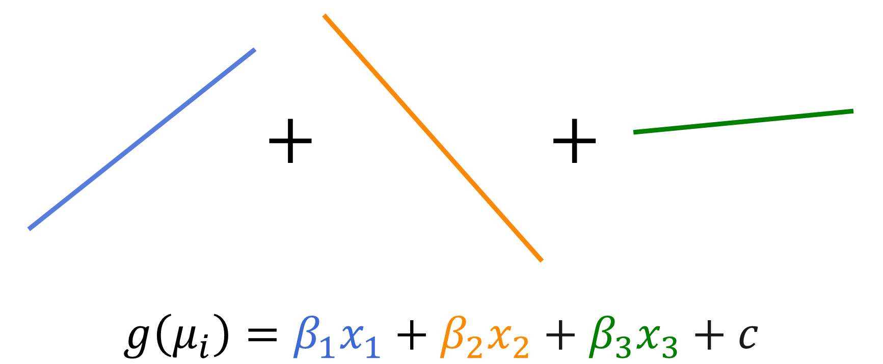
for \(i=1,\dots,n\) and \(j=1,\dots,p\), where \(x_{ij}\) is input or predictor variable j for the \(i^\text{th}\) observation or example, \(\mu_i = E[y_i]\) is the mean of the target variable distribution, \(g()\) is a link function, and \(f_j\) is a component function. GLMs further assume that each component function, \(f_j\), is a linear function of the input \(x_{ij}\), just as is assumed by the ordinary linear regression model. You can see this in Figure 1.
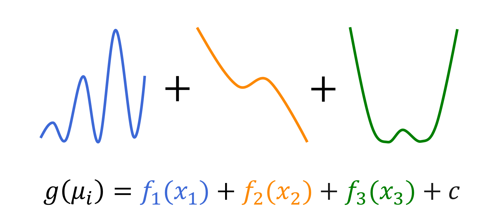
For GAMs, on the other hand, the component functions can be arbitrary nonlinear smoothing functions that the model usually estimates by using spline functions. You can see this in Figure 2.
Why use GAMs?
One of the biggest benefits of GAMs is their flexibility. Table 1 gives you some examples. Given the close relationship with GLMs, GAMs also feature the ability to model different types of data. But GAMs take this flexibility to another level by incorporating nonlinear functions that can model more complex relationships. With a linear model, you can use feature engineering, such as polynomial terms and other input transformations, to incorporate nonlinear terms into your model. However, one disadvantage to this approach is that you need to choose these transformations beforehand. This is not needed with a GAM because the smoothing components learn the relationships from the data to flexibly model nonlinearities.
| Component | Description |
| Linear predictors | Effects that involve interval or classification variables |
| Nonparametric predictors | Spline terms that involve one or two interval variables |
| Distributions | Binary, gamma, inverse Gaussian, negative binomial, normal (Gaussian), Poisson, Tweedie |
| Link functions | Complementary log-log, identity, inverse, inverse squared, log, logit, log-log, probit |
Table 1: The main parts of a GAM that contribute to its flexibility. Source: Adapted from Rodriguez & Cai (2018)
In addition, various nonparametric regression smoothing techniques can incorporate nonlinearities into your model. The vast majority of these methods are for only one input variable. So essentially they are generalizations of simple linear regression. GAMs extend these smoothing techniques to the multivariate setting while maintaining additivity. Besides the standard univariate smoothing functions for multiple inputs, a GAM can also include parametric (linear) effects, categorical inputs, and bivariate spline terms that are functions of two interval input variables.
Even with this flexibility, GAMs are still interpretable. This is an increasingly desirable feature of machine learning models. This is especially true for high-stakes applications such as health care, finance, and mission-critical systems.
Typically, you face a trade-off between model performance and model interpretability. You can see this in Figure 3. At one end of the spectrum, you have transparent models such as the ordinary linear regression model. Although it is often outperformed by other models, one of the reasons for its sustained popularity is that it is easy to understand.

At the other end of the spectrum, you have opaque machine learning models such as neural networks, gradient boosting machines (GB), random forests (RF), and support vector machines (SVM). These state-of-the-art models can predict very complex relationships extremely well. But it is difficult to interpret how the inputs affect the predictions. A highly accurate model might not be put into practice if domain experts and other stakeholders do not understand it.
GAMs occupy a sweet spot along the spectrum. GAMs can model complex relationships, but you can control the smoothness of the component functions to prevent overfitting. As a result, the predictive performance of GAMs is usually competitive with other machine learning techniques. When it comes to interpretability, the additivity of the component functions enables you to decouple the effects from the different terms. Thus, whereas opaque models are not very interpretable, with a GAM you can plot an estimated component function for an individual input to visually interpret the input’s contribution to the prediction. We will demonstrate this in the next section. Furthermore, you can easily interpret any linear effects in the GAM just like you would for a generalized linear model.
GAMs in action
Now that you have a better understanding of GAMs and their benefits, let’s see a GAM in action. The GAM node in Model Studio, part of SAS Visual Data Mining and Machine Learning in SAS Viya, provides a user interface to the GAMSELECT and GAMMOD procedures. So the node enables you to train a GAM without writing any code.
To do so, let’s revisit an example from Lamm & Cai (2020), which trains a GAM to predict the probability that a mortgage applicant will default on a loan. The complete step-by-step instructions to reproduce this analysis are in a companion SAS Community article. But for brevity, let’s skip to the results.
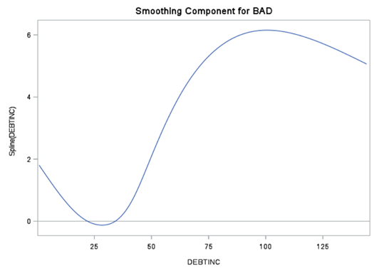
For the effects in the final model, the node’s results include smoothing component plots for the spline terms and parameter estimates for the parametric terms. For example, the results include a smoothing component plot for the Spline(Debtinc) term. Figure 4 displays this. Interpreting the results, you can see that the probability of default is generally higher for an applicant who has a high debt-to-income ratio and the relationship is nonlinear.
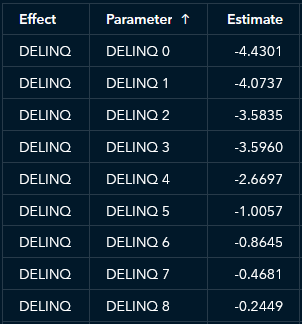
In addition, the ability to interpret the parametric effects like you would with a logistic regression model is another way in which the GAM’s results are relatively easy to understand. For example, an applicant with more delinquent credit lines has a higher predicted probability of default, on average. See Figure 5.
With Model Studio, you can also easily train other supervised learning models for comparison. Let’s compare the GAM to gradient boosting, logistic regression, neural network, and support vector machine (SVM) models. If you rank the algorithms by misclassification rate, you see that the GAM ranks second. Figure 6 displays the results.
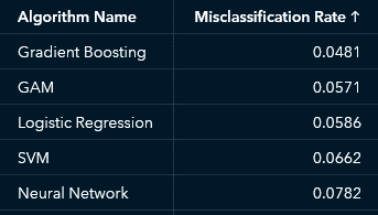
Even though the GAM has a slightly higher misclassification rate, it is more interpretable than the champion gradient boosting mode. And it still outperforms other complex models such as SVM and neural network.
Summary
GAMs extend the popular and versatile GLM framework by incorporating nonlinear terms that enable you to model even more complex relationships. GAMs are attractive because they strike a nice balance between flexibility and performance while maintaining a high degree of interpretability. In just a few clicks and keystrokes, you can train GAMs in Model Studio. Then you can compare them with other popular machine learning algorithms. As such, GAMs belong in every data scientist's toolbox.
Learn more | SAS Data Science Offerings


2 Comments
Did you try partial least squares (PROC PLS) model ? I think it is also a good model . Especial for nulti-colinearity of variables.
Hi Ksharp,
I did not try a partial least squares model for this application. My main focus was to compare a GAM to a few more modern and more opaque machine learning models to demonstrate that GAMs strike a nice balance between accuracy and interpretability.
I do agree that a PLS model is good when you have correlated inputs and would be another reasonable model for comparison. Thanks for reading the article and thanks for your suggestion!
Best,
-Brian