This post, co-authored with my colleague Ricky Tharrington, is the second of three on explaining interpretability techniques for complex models in SAS® Viya®. 

Quick introduction to Model Studio

A machine learning pipeline is a structured flow of analytical nodes, each of which performs a single data mining or predictive modeling task. Pipelines can help automate the data workflows required for machine learning, simplifying steps including, variable selection, feature engineering, model comparisons, training and deploying the model. Visibility into modeling pipelines can improve model re-use and model interpretability.

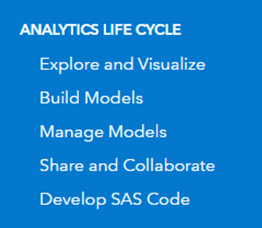
To build predictive modeling pipelines in SAS Visual Data Mining and Machine Learning, use the SAS Model Studio web-based visual interface. You can access Model Studio by selecting Build Models from the Analytics Life Cycle menu in SAS Drive, as shown in Figure 1.

An example model pipeline

When working in Model Studio, you construct pipelines by adding nodes through the point-and-click web interface. Figure 2 shows a simple Model Studio pipeline that performs missing data imputation, selects variables, constructs two logistic regression models and a decision tree model, and compares their predictive performances.

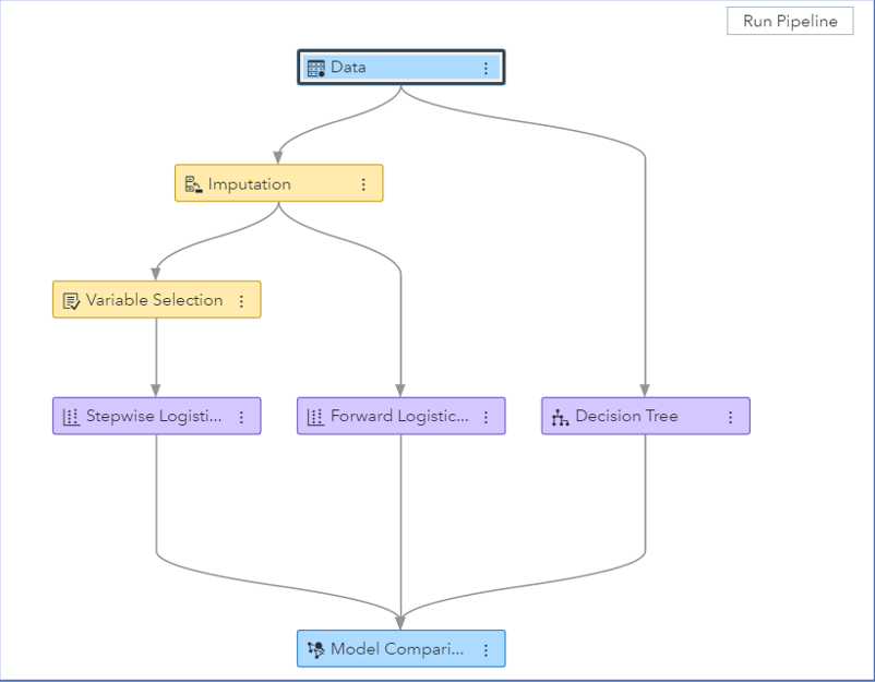
Building pipelines is considered a best practice for predictive modeling tasks because pipelines can be saved and shared with other SAS Visual Data Mining and Machine Learning users for training future machine learning models on similar data. In addition to many feature engineering capabilities, Model Studio also offers numerous ways to tune, assess, combine, and interpret models.

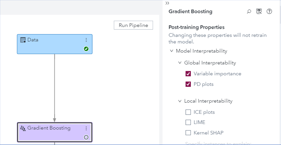
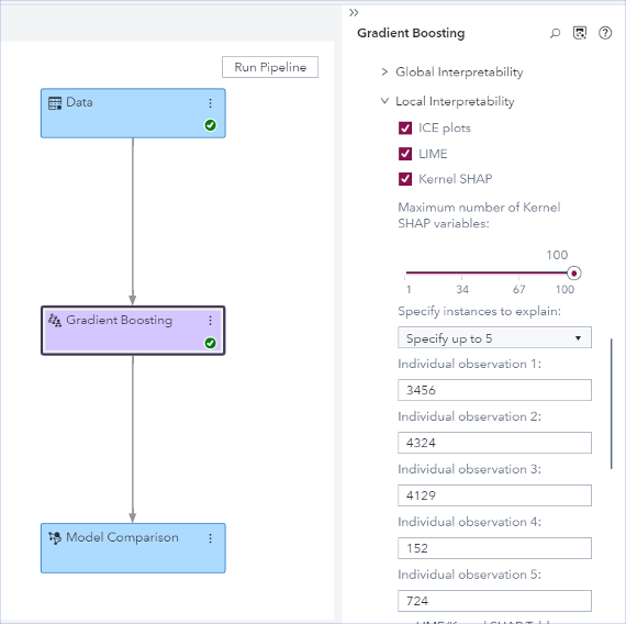
In Model Studio, model interpretability functionalities are provided as a post-training property of all supervised learning nodes. Changing post-training properties and retrieving interpretability results does not require retraining the machine learning model. Figure 3 shows the model interpretability properties for the Gradient Boosting supervised learning node.

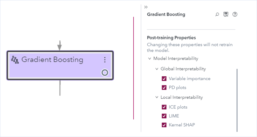
Model interpretability results are presented in a user-friendly way by decreasing the huge amount of information that might be overwhelming to users. Instead, Model Studio includes text explanations that are provided by natural language generation for an easier understanding of the results. This enables users who are less experienced with these techniques to find some meaningful insight into the relationships between the predictors and the target variable in black-box models. For more information about Model Studio, see SAS Visual Data Mining and Machine Learning: User's Guide.

An interpretability example using home equity data

Let's look at an example that demonstrates how to use SAS Model Studio for performing post-hoc model interpretability, using financial data about home equity loans. We will be building a model that determines whether loan applicants are likely to repay their loans. We will first explain how the model is built and then assess the model using various interpretability techniques.

Exploring the data and model

The data comes from the FICO xML Challenge and is contained in an anonymized data set of home equity line of credit (HELOC) applications made by real homeowners. A HELOC is a line of credit typically offered by a bank as a percentage of home equity (the difference between the current market value of a home and any liens on the home). The customers in this data set have requested a credit line in the range of $5,000–$150,000.

The goal is to predict whether the applicants will repay their HELOC account within two years. The data set has 10,459 observations for a mix of 23 interval and nominal input variables, which include predictors such as the number of installment trades with balance, the number of months since the most recent delinquency, and the average number of months in the file. The target variable is RiskPerformance, a binary variable that takes the value Good or Bad. The value Bad indicates that a customer’s payment was at least 90 days past due at some point in the 24 months after the credit account was opened. The value Good indicates that payments were made without ever being more than 90 days overdue. The data are balanced with around 52% Bad observations.

This blog post focuses on explaining model interpretability, so it skips the data preprocessing and feature generation steps. All the input variables were taken as-is, except for the variables Max Delq/Public Records Last 12 Months and Max Delinquency Ever, which were converted to strings according to the FICO data dictionary. Also, an ID variable was created to specify individual applicants when performing local interpretability.

A Model Studio project (called heloc) is created using this data set. For more information about how to create a SAS Model Studio project, see the Getting Started with SAS Visual Data Mining and Machine Learning in Model Studio section in the SAS Visual Data Mining and Machine Learning: Users Guide.

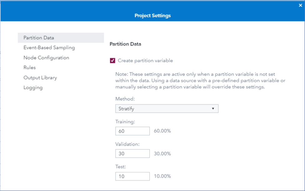
The data are partitioned by the default values of 60% for training, 30% for validation, and 10% for test sets, as shown in Figure 4.

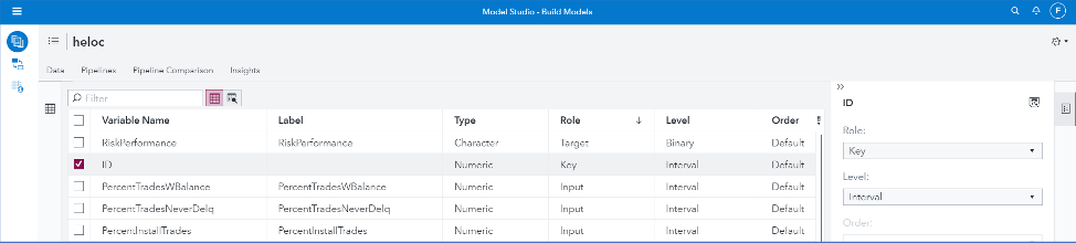
By clicking the Data tab, you can assign different roles to your input variables. Figure 5 shows that the newly created ID variable is assigned the role Key. This step is necessary if you want to specify individual predictions for local interpretability. Figure 5 also shows that the binary variable RiskPerformance is specified as the target variable.

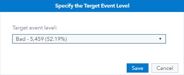
When specifying the target variable, you can choose the event level of the target variable. Figure 6 shows that the event level is specified as Bad. This means the predicted probabilities of the trained models represent the probabilities of a customer making a late payment.

To train a gradient boosting model in Model Studio, you simply need to connect the Gradient Boosting supervised learning node to the Data node. For this example, the Gradient Boosting node runs with its default settings without any hyperparameter tuning. By default, the validation set is used for early stopping to decide when to stop training boosted trees. Figure 7 shows the fit statistics of the black-box gradient boosting model.

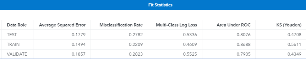
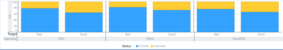
Figure 7 shows that the model’s misclassification rate on the test set is 27.8%. Figure 8 shows the corresponding event classification plot, where the larger portion of the model’s misclassification events are good applications that are predicted as bad.

To improve prediction accuracy, you can perform a hyperparameter search for your gradient boosting model by turning on the Perform Autotuning property, which is available in all the supervised machine learning nodes in Model Studio. To learn more about automated hyperparameter tuning functionality in SAS Viya, see Koch et. al. (2018).

Global interpretability

This section shows how you can request and view global interpretability plots.
Figure 9 shows the checkboxes you use to enable a node’s global interpretability methods (variable importance and partial dependence plots) in Model Studio. Note that since the model interpretability techniques covered here are post-hoc, they are done after training the gradient boosting model. This means that unless you change any model training properties, changing a post-training property such as model interpretability does not require retraining the model.

Variable importance

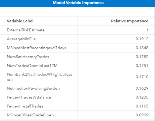
The model variable importance table in Figure 10 shows the ranking of the importance of the features in the construction of the gradient boosting model.

Partial dependence plots

In Model Studio, by default partial dependence plots are generated for the top five variables in the variable importance table. Figure 11 and Figure 12 show the partial dependency plots for the top two variables. In Figure 11, you can see that the predicted probability of payments being 90 days overdue decreases monotonically as the external risk estimate value increases. A text box to the right of the graph explains the graph by using natural language generation (NLG) in SAS Viya. All model interpretability plots have NLG text boxes. These explanations help clarify the graphs and are especially useful if you are not familiar with the graph type.

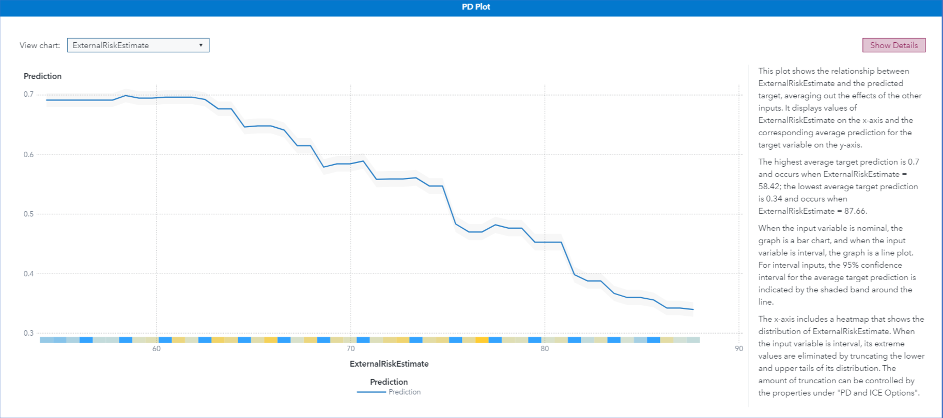
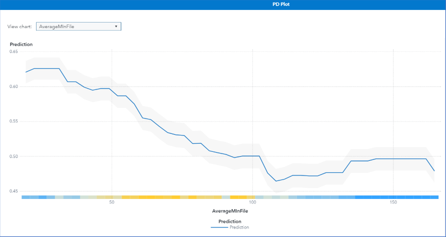
Figure 12 shows that the predicted probability of Bad payments decreases gradually as the applicant’s number of months in file increases from 50 months to 100 months. This is expected because applicants who have a longer credit history are deemed less risky. The heat map on the X-axis shows that not many observations have an average number of months in file greater than 100. After the number of months in file reaches 100, the probability of Bad payments first increases slightly and then flattens because the model has less information in this domain. Hence, you should be cautious in explaining the part of the plot where the population density is low.

Local interpretability

Local interpretability helps you understand individual predictions. Figure 13 shows the Gradient Boosting node’s options for requesting local interpretability (ICE, LIME, and Kernel SHAP) for five applicants who are specified by their IDs. This identification variable should have unique values and must be specified to have the role Key (only one variable can have this role) on the Data tab.

ICE plots

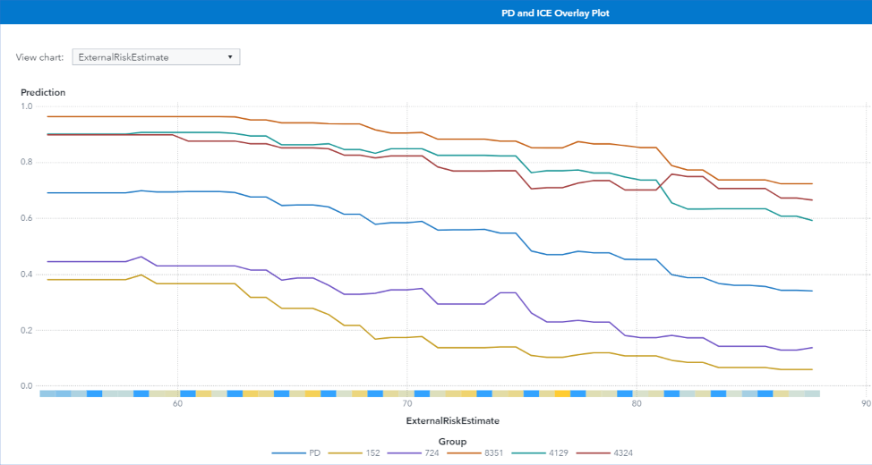
Figure 14 shows the five ICE plots for the specified observations for the external risk estimate input variable. The change in the model’s prediction for each of these observations decreases as the external risk estimate increases, which matches the behavior that is seen in the partial dependence curve (shown in blue). Each observation is affected by the external risk estimate slightly differently. For observation 152, there is a steep decline in the model’s predicted probability of late payment when the external risk estimate is between 60 and 70, whereas for observation for 4129, the decline is more gradual between 60 and 70 and is steeper after 70.

True positive prediction of high-risk (LIME Explanation)

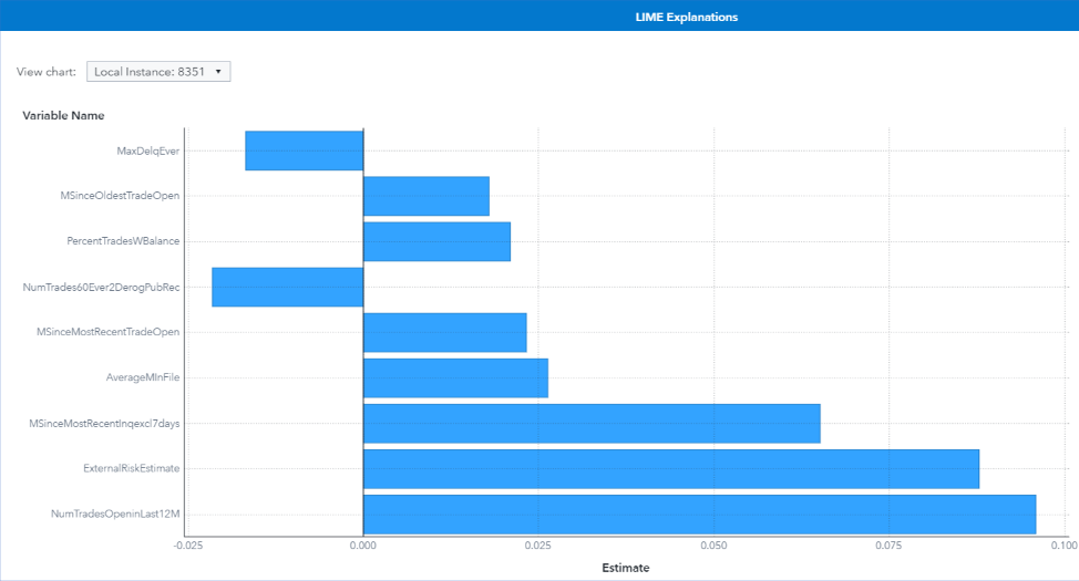
Figure 15 shows the LIME explanation of the prediction of the black-box gradient boosting model for instance 8351. Gradient boosting models predict this instance as a high-risk HELOC application with a predicted probability of 0.965.

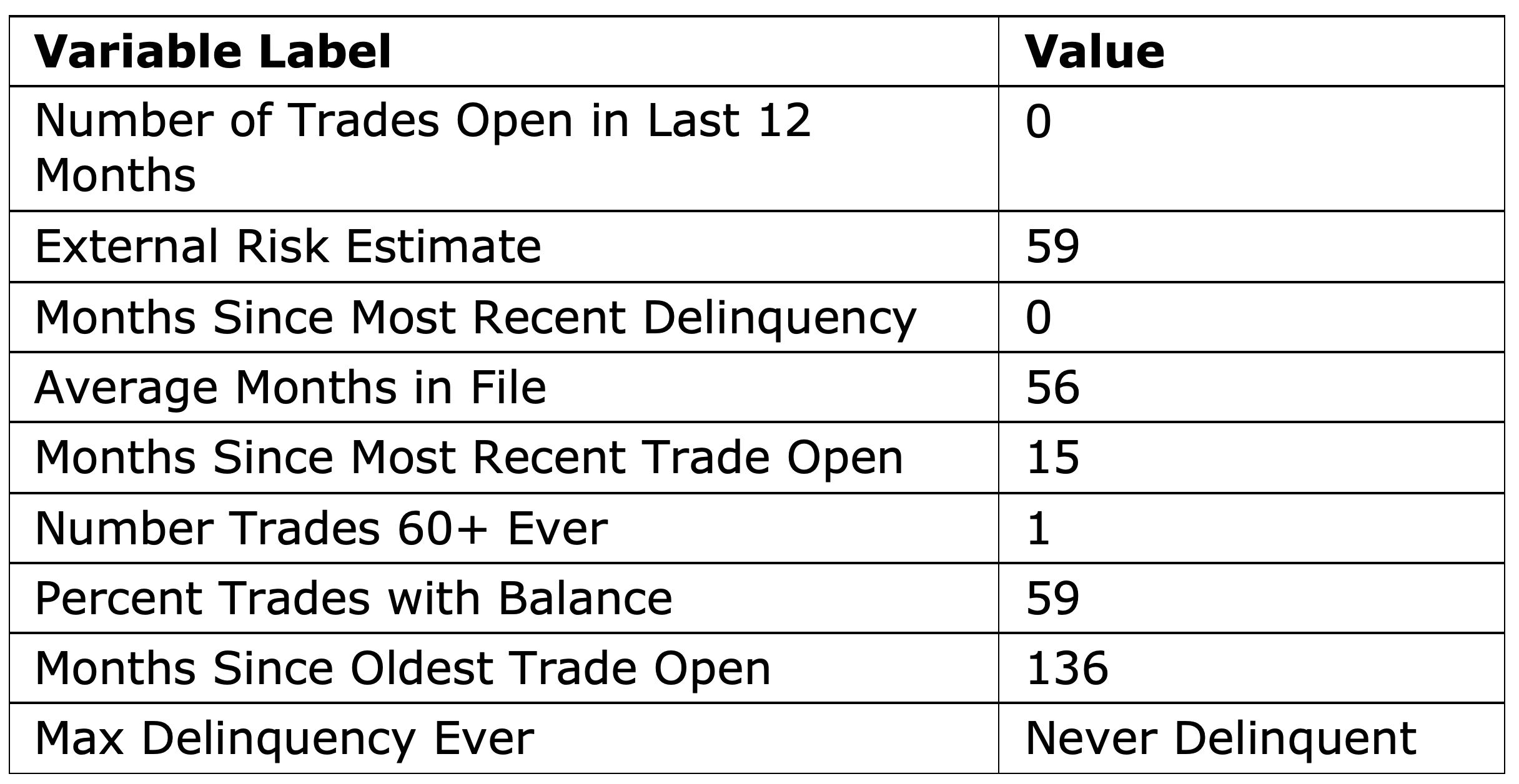
When LIME is implemented, a local model is fit after converting each feature into a binary feature according to its proximity to the explained observation. Therefore, the coefficients in the LIME explanation represent the impact of the observed feature values of the instance. The feature values of instance 8351 are shown in Table 1.

The LIME explanation for instance 8351 shows that Number Trades 60+ Ever=1 and Max Delinquency Ever=Never Delinquent decrease the risk of default, whereas all other predictors increase the risk of default.

False positive prediction of high risk (Kernel SHAP explanation)

Figure 16 shows the Kernel SHAP explanation of the prediction of the black-box gradient boosting model for instance 4129. The ground truth for this instance is Good, but the models output a high probability (0.904) of predicting it as Bad.

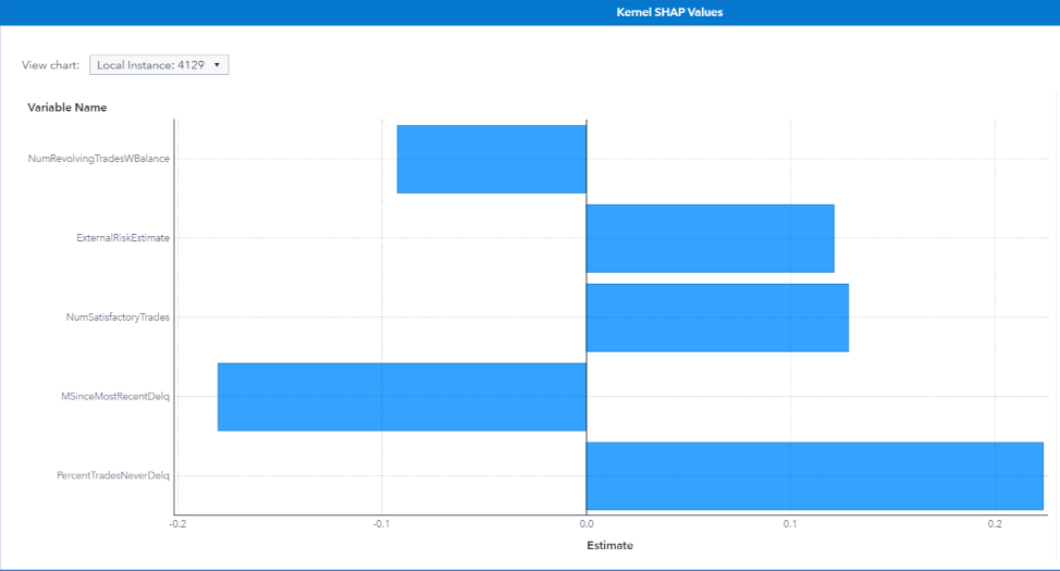
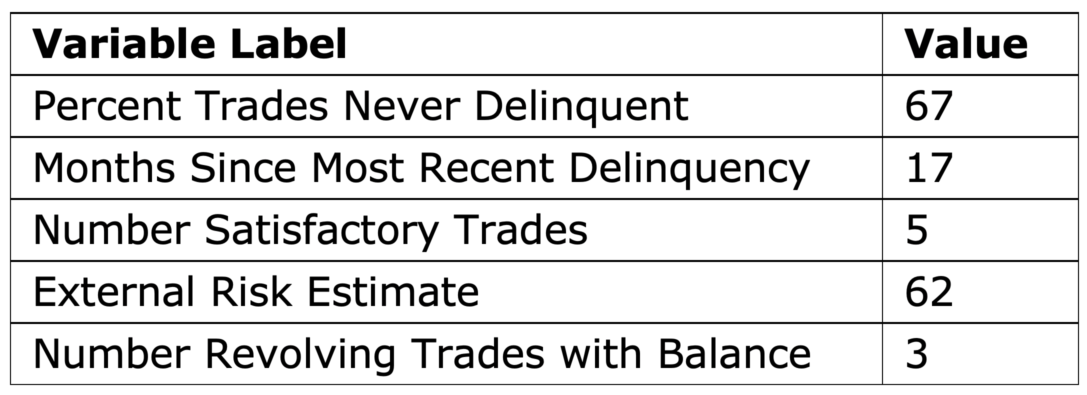
The Kernel SHAP explanation in Figure 16 and the feature values in Table 1 show that the features that contribute most toward increasing the high risk of late payments are Percent Trades Never Delinquent=67, Number Satisfactory Trades=5, and External Risk Estimate=62. Even though the model has such a high confidence in its prediction, the same confidence is not seen by examining the top five Kernel SHAP explanations, which can be used as a warning sign for this false prediction.

Read our quick guide: The Machine Learning Landscape