Portfolio Optimization using SAS and Python

Introduction

Analytics can be categorized into four levels: descriptive, diagnostic, predictive, and prescriptive. Descriptive analytics explore what happened, diagnostic analytics examine why something happened, and predictive analytics imagine what will happen. Today, we will focus on the final level, prescriptive analytics, which tries to find the best possible outcome. Specifically, we will focus on using optimization to select a stock portfolio that maximizes returns while taking risk tolerance into account.

Before we can solve our optimization problem, we must first set it up. An optimization problem consists of several pieces, including the objective function, the decision variables, and the constraints. The objective function is our goal and takes the form of a minimization or maximization. Our goal is to maximize expected return. Decision variables are the factors we have control over to change the value of the objective function. In our example, our decision variables are the proportion of our portfolio our potential stocks hold. Finally, constraints are bounds on our optimal solution based on what is possible. For our problem, we cannot hold a negative proportion of stock, we cannot invest more money than we have, but we will invest all of the money in our portfolio, and we cannot exceed our risk threshold.

Enter sasoptpy

As I was studying for the SAS Forecasting and Optimization Specialist certification exam, the sasoptpy open source package was released. This is a Python package providing a modeling interface for SAS Viya Optimization solvers. It supports Linear Problems (LP), Mixed Integer Linear Problems (MILP), Non-Linear Problems (NLP), and Quadratic Problems (QP). To solidify my studies, I took the portfolio optimization problem and translated it into Python using sasoptpy in this Jupyter Notebook.

Portfolio Optimization using SAS and Python

I started by declaring my parameters and sets, including my risk threshold, my stock portfolio, the expected return of my stock portfolio, and covariance matrix estimated using the shrinkage estimator of Ledoit and Wolf(2003). I will use these pieces of information in my objective function and constraints. Now I will need SWAT, sasoptpy, and my optimization model object.

import swat
import sasoptpy as so
conn = swat.CAS('localhost', 5570, authinfo='~/.authinfo', caslib="CASUSER")
m = so.Model(name='portfolio_opt', session=conn)

Next, I declared my decision variables, which are the proportions each stock will hold in my optimal portfolio. When declaring my decision variables, I added a lower bound of zero to ensure that I will have non-negative proportion values.

proportion=m.add_variables(ASSETS, name='proportion', lb=0)

Then I declared my constraints. My first constraint ensures that the proportion of stocks in my portfolio sum to one. This means I will invest all of my money, but not more.

money_con = m.add_constraint(
        (so.expr_sum(proportion[i] for i in ASSETS) == 1), 
        name='money_con')

I used the covariance matrix to constrain my risk, as measured by variance, such that is was smaller than my risk threshold.

risk_con = m.add_constraint(
        (so.expr_sum(COVAR.at[i,j]*proportion[i]*proportion[j] for i in ASSETS for j in ASSETS) <= RISK_THRESHOLD), 
        name='risk_con')

Finally, I created my objective function to maximize my expected value.

total_return = m.set_objective(so.expr_sum(RETURNS['EXPECTED_RETURNS'][i]*proportion[i] for i in ASSETS),
                               sense=so.MAX, 
                               name='total_return')

Now solving the optimization problem once it is set up is a piece of cake. SAS will automatically decide which optimization algorithm to used based on my problem.

sol = m.solve()

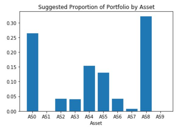
And just like that, an optimal solution was found using the Interior Point Direct algorithm with a potential expected returned of 10.14 with the given stock proportions.

The full problem set-up, additional information, completed code and results are available in my Jupyter Notebook!

Conclusion and learning more

We used sasoptpy to set up an optimization problem to select our stock portfolio for us. This was an over-simplified example as should not be used as investment advice, but this was only one use case for sasoptpy. Other really cool use cases to explore are more efficiently allocating political campaign funds, optimization of shipping logistics, solving the Stigler diet problem, and building the best sports teams.

If you are interested in learning more about optimization, check out the Optimization Concepts for Data Science and Artificial Intelligence course. It's a great course to take, especially if you are hoping to grab your SAS Professional Certification in Artificial Intelligence and Machine Learning!