Bayesian optimization in SAS

My colleague Wayne Thompson has written a series of blogs about machine learning best practices. In this series' fifth post, Autotune models to avoid local minimum breakdowns, Wayne discusses two autotune methods, grid search and Bayesian optimization. According to another colleague’s paper, Automated Hyperparameter Tuning for Effective Machine Learning, Bayesian optimization is currently popular for hyperparameter optimization. Recently, I read a post on Github which demonstrated the Bayesian optimization procedure through a great demo using Python, and I wondered if I could build the same with the SAS matrix language, SAS/IML. In this article, I will show you how Bayesian optimization works through this simple demo.

Revisit Bayesian optimization

Bayesian optimization builds a surrogate model for the black-box function between hyperparameters and the objective function based on the observations and uses an acquisition function to select the next hyperparameter.

1. Surrogate model

Functions between hyperparameters and objective function are often black-box functions, and Gaussian Process regression models are popular because of its capability to fit black-box functions with limited observations. More details about Gaussian Process regression, please refer to the book Gaussian Processes for Machine Learning.

2. Acquisition function and Location Propose function

The acquisition function evaluates points in the search space and the location propose function finds points which will likely lead to maximum improvement and are worth trying. The acquisition function trades off exploitation and exploration. Exploitation selects points having high objective predictions, while exploration selects points having high variance. There are several acquisition functions, and I used expected improvement, which is the same as in the GitHub post that I'm modeling.

3. Sequential optimization procedure

Bayesian optimization is a sequential optimization procedure. The algorithm follows:

For t=1, 2, ... do

Find the next sampling point by optimizing the acquisition function over the Gaussian Process (GP).
Obtain a possibly noisy sample from the objective function.
Add the sample to the previous samples and update the GP.

end for

Implementation with SAS/IML

1. Gaussian Process Regression

In the code, the SAS macro gpRegression is used to fit a Gaussian Process regression model through maximizing the marginal likelihood. More details, please read chapter 5 of Gaussian Processes for Machine Learning.

2. Bayesian optimization

The SAS macro bayesianOptimization includes two functions: the acquisition function and location propose function.

3. Visualization

Finally, the macro plotAll shows you the step-by-step optimization procedure visually.

The code for these macros and following demo codes are available on my GitHub project.

Demo implementation with SAS/IML

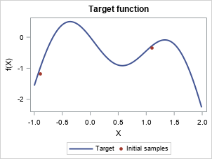
proc iml;
   %gpRegression;
   %bayesianOptimization;  
 
   * Target function;
   start f(X, noise=0);
       return (-sin(3*X) - X##2 + 0.7*X + noise * randfun(nrow(X), "Normal"));
   finish;   
 
   * Search space of sampling points;
   X = T(do(-1, 1.99, 0.01));
   call randseed(123);
   Y = f(X, 0);   
 
   * Initialize samples;
   X_train ={-0.9, 1.1};
   noise = 0.2;
   Y_train = f(X_train, noise);  
 
   * Initial parameters of GP regression model;
   gprParms = {1 1 0};
 
   * Max iterations for sequential Bayesian Optimization;
   n_iter = 15;
   do i=1 to n_iter;
      * Update Gaussian process with existing samples;
      gprParms = gprFit(gprParms);
 
      * Obtain next sampling point from the acquisition function (acquisition);
      proposeResults = proposeLocation(X, X_train, Y_train, gprParms);
      X_next = proposeResults$"max_x";
      if X_next=. then leave;
 
      * Obtain next noisy sample from the objective function;
      Y_next = f(X_next, noise);
 
      * Add sample to previous samples;
      X_train = X_train//X_next;
      Y_train = Y_train//Y_next;  
 
      * Save all proposed sampling points into a matrix;
      allProposed = allProposed//(j(1, 1, i)||X_next);
   end;
 
   * Save all proposed sampling points into a SAS dataset;
   create allProposed from allProposed [colname={"Iteration" "X"}];
   append from allProposed;
   close allProposed;
run;
quit;

Visualize the step-by-step Bayesian optimization procedure

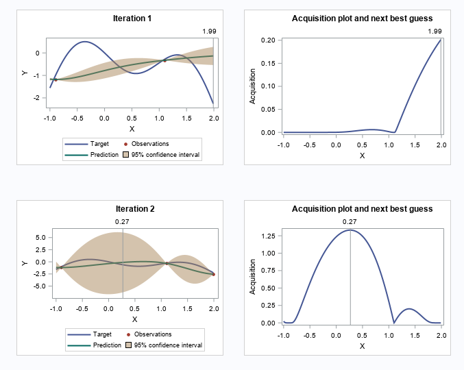
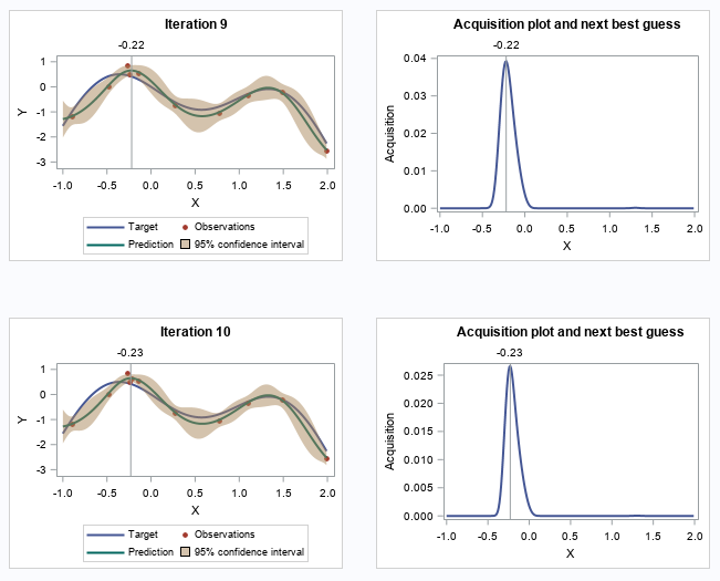
Figure 1: Target function and initial two samples.

Figure 2: Proposed location and acquisition function plot of the first two iterations.

Let's skip to the last two iterations.

Figure 3: Proposed location and acquisition function plot of the last two iterations.

To demonstrate the whole procedure visually, I created an animation file.

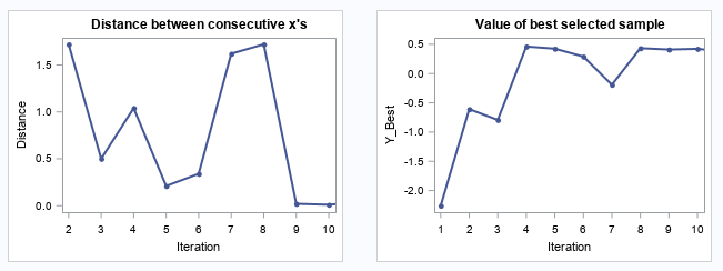
Figure 4: Animation of the step-by-step optimization.

The following two plots show the convergence trend along with iterations. The left plot displays distance between consecutive proposed points by iteration, and starting from iteration 9, the distance is close to zero. The right plot shows the value of the best selected sample, and starting from iteration 8, the values almost didn’t change.