When building models, data scientists and statisticians often talk about penalty, regularization and shrinkage. What do these terms mean and why are they important?

According to Wikipedia, regularization "refers to a process of introducing additional information in order to solve an ill-posed problem or to prevent overfitting. This information usually comes in the form of a penalty for complexity, such as restrictions for smoothness or bounds on the vector space norm.”

Shrinkage can be thought of as "a penalty of complexity." Why? If we set some parameters of the model to exactly zero, then the model is effectively shrunk to have lower-dimensionality and less complex. Analogously, if we use a shrinkage mechanism to zero out some of the parameters or smooth the parameters (the difference of parameters will not be very large), then we are decreasing complexity by reducing dimensions or making it more continuous.

Why do we want to use shrinkage mechanism in training data? In real life, we often encounter problems where we have less data but a lot of features in our problem. These problems become ill-posed, meaning no unique solution can be found.

In fact, without using shrinkage, we can find a lot, if not unlimited, solutions to them. And the learned model from such data sets will often over fit. It will fit the training data perfectly but it does not generalize well to the unseen data (See Figure 1).

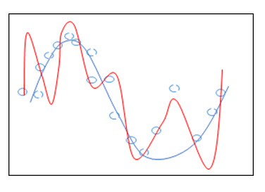
Before we jump into this figure, let us first explain what the figure means. In Figure 1, the blue line is the true underlying model. The blue circles are noisy samples drawn from the model. We separate all samples into two groups -- training samples denoted by blue solid circles and testing samples represented by blue dotted circles. Our problem can be expressed as:
\begin{equation}\label{eq:LS}
\hat\beta =\mathrm{arg}\max_{\beta}\sum_{j=1}^{n}(y_j-\sum_{i=1}\beta_i\phi_i(x_j))^2
\end{equation}
where $\beta_i$ is the parameter that we want to learn, $x_j$ is the $i$th data point and $y_i$ is the $i$th predicted value in the training data set.

Assume that the red line is the regression model we learn from the training data set. It can be seen that the learned model fits the training data set perfectly, while it cannot generalize well to the data not included in the training set. There are several ways to avoid the problem of overfitting.

To remedy this problem, we could:

• Get more training examples.
• Use a simple predictor.
• Select a subsample of features.

In this blog post, we focus on the second and third ways to avoid overfitting by introducing regularization on the parameters $\beta_i$ of the model.

Three types of regularization are often used in such a regression problem:
• ${l}_2$ regularization (use a simpler model)
• ${l}_1$ regularization (select a subsample of features)
• ${l}_{12}$ regularization (both)

${l}_2$ regularization, which adds a penalty of ${l}_2$ norm on the parameters $\beta_i$, encourages the sum of the squares of the parameters $\beta_i$ to be small. The original problem is transformed to the ridge regression, which can be expressed as
\begin{eqnarray}\label{eq:ridge}
\hat\beta = \mathrm{arg}\max_{\beta}\sum_{j=1}^{n}(y_j-\sum_{i=1}\beta_j\phi_i(x_j))^2+\lambda\sum_i\beta_i^2
\end{eqnarray}
where the shrinkage parameter $\lambda$ need be tuned via cross-validation.

The ${l}_2$ regularization can be explained from a geometric perspective. As shown in Figure 2, the residual sum of squares has elliptical contours, represented by a black curve. The ${l}_2$ constraint is represented by the red disk. The first point where the elliptical contours hit the constraint region is the solution of ridge regression. ${l}_2$ regularization will keep all predictors by jointly shrinking the corresponding coefficients. It also reduces the possible solution to those points in the intersection of two contours. The intersection is a much smaller set than the original parameter space. Therefore it reduces the complexity of the model and smooths it.

$l_1$ regularization, instead, which uses a penalty term of ${l}_1$ norm, encourages the sum of the absolute values of the parameters to be small. Problem (\ref{eq:LS}) then becomes Lasso regression, which can be expressed as:
\begin{eqnarray}\label{eq:L1}
\hat\beta =\mathrm{arg}\max_{\beta}\sum_{j=1}^{n}(y_j-\sum_{i=1}\beta_j\phi_i(x_j))^2+\lambda\sum_i|\beta_i|
\end{eqnarray}

Unlike the ${l}_2$ regularization, the ${l}_1$ constraint is represented by a red diamond, seen in Figure 3. The diamond has corners; if the solution occurs at a corner, then it has one parameter $\beta_j$ equal to zero.

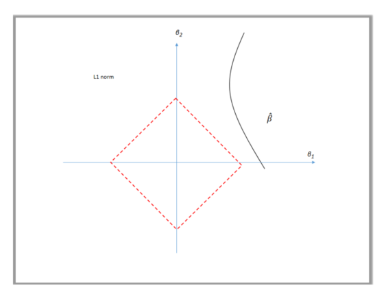
Lasso regression uses this shrinkage mechanism to zero out some parameters $\beta_i$ and de-select the corresponding features $\phi_i(x_j)$. Due to its strong tends of setting some parameters to zeros, it is often used to select features when we know that some features are really very sparse.

Elastic net regularization is a tradeoff between ${l}_2$and ${l}_1$ regularization and has a penalty which is a mix of $l_1$ and $l_2$ norm. It can perform the function of feature selection while still not imposing too much sparsity on the features (discarding too many features) by imposing a mixture of ${l}_2$ and ${l}_1$ regularization on parameters $\beta_i$, seen in equ.(\ref{eq:L12}).
\begin{eqnarray}\label{eq:L12}
\hat\beta =argmax_{\beta}\sum_{j=1}^{n}(y_j-\sum_{i=1}\beta_j\phi_i(x_j))^2+\lambda_1\sum_i|\beta_i|+\lambda_2\sum_i\beta_i^2
\end{eqnarray}

The selection of different penalties depends on problems. If the signals are truly sparse, then $l_1$ or $l_{12}$ penalty can be used to select the hidden signals from noisy data while it is almost impossible for $l_2$ to fully recover the the sparse signals. For problems with features not sparse at all, I often find the $l_2$ regularization often outperforms $l_1$ regularization. In the prediction application, ridge regression with $l_2$ is more common and often recommended for many modeling. However in the case where you have many features and want to reduce the complexity of the model by de-selecting some features, you may want to impose $l_1$ penalty or go for more of a balanced approach like elastic net.

Therefore, it is best to collect as many samples as possible. Even with a lot samples, a simpler model with $l_2$ regularization will often perform better than other choices.

For more on regularization, be sure to read these posts in the SAS Community:

• Tuning Matters: An Example of LASSO Tuned via Validation Data and Cross Validation
• Tip: Top five reasons for using penalized regression for modeling your high-dimensional data