In our previous post, Econometric and statistical methods for spatial data analysis, we discussed the importance of spatial data. For most people, understanding that importance is relatively easy because spatial data are often found in our daily lives and we are all accustomed to analyzing them. We can all relate to the first law of geography—“Everything is related to everything else, but near things are more related than distant things”—and we can agree that our interaction with close things around us plays an important role in our decision process. Applications of spatial data in our daily lives are often seamless, and you could argue that we are all spatial statisticians and econometricians without even realizing it. Although most human beings have an innate ability to incorporate spatial information, computer-based analytics need to be given tools to include such information in their analyses. SAS/ETS 14.2 introduces one such tool, the SPATIALREG procedure, which enables you to include spatial information in the analysis and improve the econometric inference and statistical properties of estimators.
In this post, we discuss how you can use the SPATIALREG procedure to analyze 2013 home value data in North Carolina at the county level. The five variables in the data set are county (county name), homeValue (median value of owner-occupied housing units), income (median household income in 2013 in inflation-adjusted dollars), bachelor (percentage of people with bachelor’s degree or higher who live in the county), and crime (rate of Crime Index offenses per 100, 000 people). The data for home values, income, and bachelor’s degree percentages in each county were obtained from the website of the United States Census Bureau and computed using the 2009–2013 American Community Survey five-year estimates. Data for crime were retrieved from the website of North Carolina Department of Public Safety. For the purpose of numerical stability and interpretation, all five variables are log-transformed during the process of data cleansing. We use this data set to demonstrate the modeling capabilities of the SPATIALREG procedure and to understand the impact of household income, crime rate, and education attainment on home values.
As a preliminary data analysis, we first show a map of North Carolina that depicts the county-level home values in Figure 1. It is easy to see that the home values tend to be clustered together. Higher values are found in the coastal, urban, and mountain areas of North Carolina and lower home values can be found in rural areas. Home values of neighboring counties more closely resemble each other than home values of counties that are far apart.
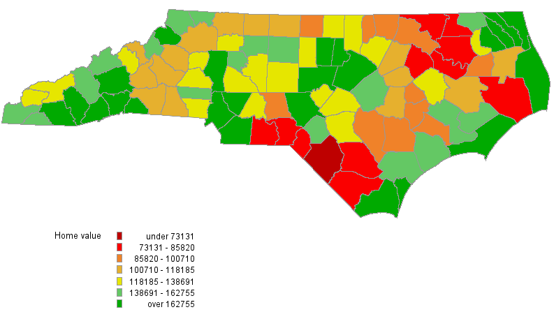
From a modeling perspective, findings from Figure 1 suggest that the data might contain a spatial dependence, which needs to be accounted for in the analysis. In particular, an endogenous interaction effect might exist in the data—home values tend to be spatially correlated with each other. PROC SPATIALREG enables you to analyze the data by using a variety of spatial econometric models.
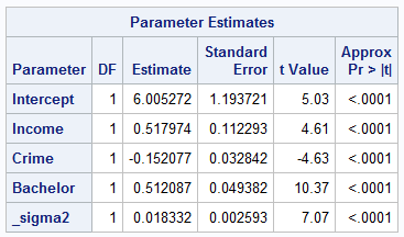
To lay the groundwork for discussion, you can start the analysis with a linear regression. For this model, the value of Akaike’s information criterion (AIC) is –106.12. The results of parameter estimation from a linear regression model, shown in Table 1, suggest that three predictors—income, crime, and bachelor—are all significant at the 0.01 level. Moreover, crime exerts a negative impact on home values, indicating that high crime rates reduce home values. On the other hand, both income and bachelor have positive impacts on home values.
Figure 2 provides the plot of predicted homeValue from the linear regression model. Although the comparison of Figure 1 and Figure 2 might suggest that predicted homeValue from the linear regression model captures the general pattern in the observed data, you need to be careful about some underlying assumptions for linear regression. Among those assumptions, a critical one is that the values of the dependent variable are independent of each other, which is not likely for the data at hand. As a matter of fact, both Moran’s I test and Geary’s C test suggest that there is a spatial autocorrelation in homeValue at the 0.01 significance level. Consequently, if you ignore the spatial dependence in the data by fitting a linear regression model to the data, you run the risk of false inference.
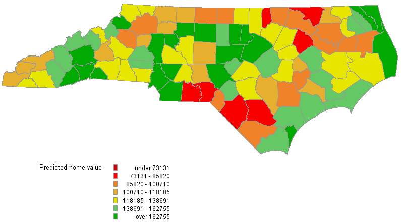
using a linear regression model
Because of the spatial dependence in homeValue, a good candidate model to consider might be a spatial autoregressive (SAR) model for its ability to accommodate the endogenous interaction effect. You can use PROC SPATIALREG to fit a SAR model to the data. Before you proceed with model fitting, you need provide a spatial weights matrix. Generally speaking, a spatial weights matrix summarizes the spatial neighborhood structure; entries in the matrix represent how much influence one unit exerts over another.

The spatial weights matrix specification is of vital importance in spatial econometric modeling. Despite many different ways of specifying such a matrix, results can be sensitive to the choice of a spatial weights matrix. Without delving into the nitty-gritty of such choice, you can simply define two counties to be neighbors of each other if they share a common border. After creating the spatial weights matrix, you can feed it into PROC SPATIALREG and run a SAR model. Table 2 presents the results of parameter estimation from a SAR model.
For this model, the value AIC is –110.79. The regression coefficients that correspond to income, crime, and bachelor are all significantly different from 0 at the 0.01 level of significance. Both income and bachelor exhibit a significantly positive short-run direct impact on home values. In contrast, crime rate shows a significantly negative short-run direct impact on home values. In addition, the spatial autoregressive coefficient ρ is significantly different from zero at 0.01 level, suggesting that there is a significantly positive spatial dependence in home values.
Figure 3 shows the predicted values for homeValue from the SAR model. Comparing Figures 1 and 3 suggest that the fitted home values capture the trend in the data reasonably well.

In this post, we introduced the SPATIALREG procedure, fit a SAR model, and compared predicted values from the SAR model to those from linear regression. Even though the SAR model presented an improvement over the linear model in terms of AIC, many other models are available in the SPATIALREG procedure that might provide even more desirable results and more accurate predictions. These models include the spatial Durbin model (SDM), spatial error model (SEM), spatial Durbin error model (SDEM), spatial autoregressive confused (SAC) model, spatial autoregressive moving average (SARMA) model, spatial moving average (SMA) model, and so on. In the next post, we will discuss their features and show you how to select the most suitable model for the home value data set. We will also be giving a talk, "Location, Location, Location! SAS/ETS® Software for Spatial Econometric Modeling," at the SAS Analytics Experience conference September 12-14, 2016 in Las Vegas, so stop by and let's talk spatial!
This post was co-written with Jan Chvosta.


2 Comments
Very informative information, i was using ARCGIS for SAR. Could you please also blog on Spatial Weights Matrix, very keen in understand how to create this Matrix
Thanks for your comment, Rajendra! We will consider writing a blog post on how to create a spatial weights matrix in the near future. Please stay tuned.