Welcome to the first post in my series Getting Started with Python Integration to SAS Viya for Predictive Modeling.

I'm going to dive right into the content assuming you have minimal knowledge on SAS Cloud Analytic Services (CAS), CAS Actions and Python. For some background on these subjects, refer to the following:

CAS Actions and Action Sets - a brief intro - a quick introduction about the distributed CAS server in SAS Viya
Getting Started with Python Integration to SAS Viya Series - more information on connecting and loading data into CAS

Now let's get started and learn how to explore the data before fitting a model. Before fitting any models, it is essential to inspect the data and explore questions such as: How accurate is the data? Are there missing values? Is there a possibility of incorrect or faulty information in some columns? Answering these queries can help you ensure that your model works correctly.

Load Data

For this Blog series I will use the home_equity.csv file from the SAS Viya example data library. For additional information on loading data into CAS see Loading a Client-Side CSV File into CAS or Loading Server-Side Files into Memory.

After making a connection to CAS (for more information on connecting to CAS see Making a Connection) load the Home Equity data into memory on CAS. Here the word conn is our connection object to CAS.

HomeEquity = conn.upload_file("https://support.sas.com/documentation/onlinedoc/viya/exampledatasets/home_equity.csv",   
                     casOut={"name":"HomeEquity",
                             "caslib":"casuser",
                             "replace":True})

The data is now not only loaded onto the CAS server, but also into CAS memory, and ready to be explored.

HomeEquity is our CAS table object and will be how I refer to and access the data in the code below.

Before I start building any predictive model, there are always certain questions I make sure to ask regarding my data.

How many rows and columns?
What type of columns (numeric or categorical)?
What do the values look like?
Are there any issues I can see visually (think dirty data)?
Are there any missing values?

Python (pandas) and CAS Actions provide us with an effective way to execute these tasks. Of course, there are multiple approaches available depending on your preferences. In this tutorial, I will be utilizing CAS Actions primarily because the requests are processed quickly and efficiently on a dedicated server when dealing with huge data sets.

How Many Columns in the Data

To answer the question on the number of columns in the data, let’s use the table action set and the recordCount action.

conn.table.recordCount(table='HomeEquity')

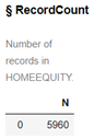
This data has 5,960 rows.

Traditional Python methods are available as well. If you want both the number of columns and number of rows, use the shape method.

display(HomeEquity.shape)

HomeEquity has not only 5,960 rows but also 18 columns.

How to Look at Column Information

Let's delve deeper and investigate which columns our data contains and what types of data each holds. Use the table action set and the columnInfo action.

HomeEquity.table.columnInfo()

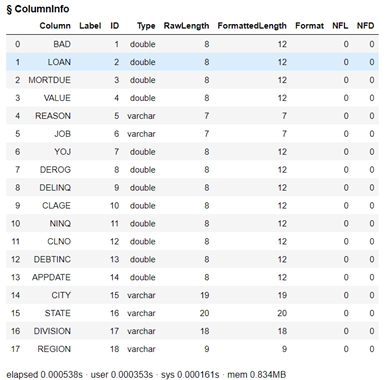
Of the 18 columns, we have 6 that are categorical, represented by varchar and the other 12 are numerical represented by double. Some of the latter may be categorical as well, but we will have to do further exploration to determine that. Let’s look.

Review the Data

Let's take a closer look at the values of the columns. By utilizing both the table action set and fetch action, we can glance at the initial five rows with ease.

conn.table.fetch(table='HomeEquity', to=5)

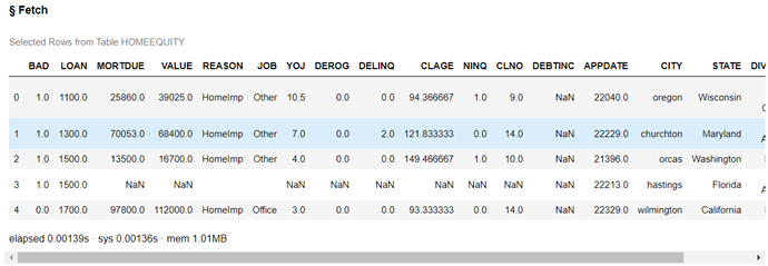
When I look at BAD, I notice its values are 1 and 0. However, REASON and JOB have only one value each. Are there any additional values for these three columns?

I also notice a portion of data is missing, represented as NaN (in numerical form) or an empty field for character values.

It appears that APPDATE is a SAS Date, and we will dive into how to work with Dates in the next post.

Descriptive Statistics

Using descriptive statistics will help us see more of the information in the data: the number of values for categorical, the number of missing for all the columns, and the mean, minimum, and maximum for numerical columns.

Using three different actions (distinct, freq, and summary) from the simple action set, let’s explore the data values further.

Distinct action

The distinct action gives us both the number of unique values for each column and the number of missing values.

conn.simple.distinct(table = HomeEquity)

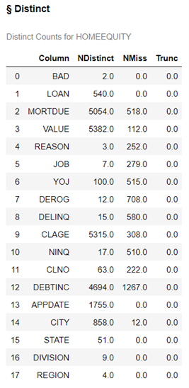
We have 5 columns with less than 10 unique values, these are potential categorical inputs (often referred to as nominal) for our model. For categorical inputs, we want to minimize the number of levels because more levels mean more complexity for our models.

We also have several columns with missing values. Part 3 of this series will address how to work with these columns.

Freq action

The freq action gives us the frequency of each of the unique values for the individual columns. In this example the inputs = option is used to only look at the frequency for the categorical columns with seven or fewer levels. To keep it simple we will use REGION instead of DIVISION to represent a geographic element in our model.

As you can imagine using freq on all columns would produce a lot of output. 😊

conn.simple.freq(table = 'HomeEquity',
    inputs = ["BAD","REASON","JOB","REGION"])

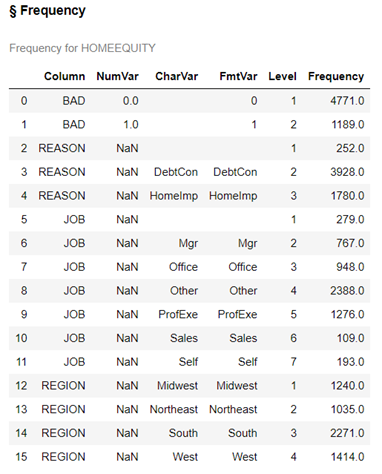
This output shows that we have missing values for REASON and JOB, but not BAD and REGION. This data also reveals that the columns aren't sparse, as there is a decent proportion of rows for each value.

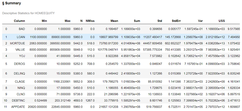
Summary action

The summary action only creates summary descriptive statistics for numerical columns because the mean of a categorical doesn’t make sense 😊.

In this example, all the summary statistics are calculated and include the minimum (MIN), maximum (MAX), number of rows (N), number missing (NMISS), mean, sum, standard deviation (STD), standard error (STDERR), variance (VAR), Uncorrected Sum of Squares (USS), Corrected Sum of Squares (CSS), Coefficient of variation (CV), t-statistic (TValue), the p-value for statistic (ProbT), Skewness, and Kurtosis.

conn.simple.summary(table='HomeEquity')

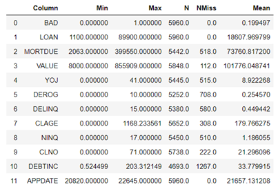
With the subSet= option, we quickly get a clearer picture of the descriptive statistics of interest.

conn.simple.summary(table='HomeEquity',
                    subSet=["N","NMISS","MEAN","MIN","MAX"])

By examining the descriptive statistics, we can detect any dirty data present. Thankfully, there appears to be none here! We'll also take note of missing values in each column which is something that will get discussed during Part 3 of this series.

Advanced statistics such as Skewness and Kurtosis may come into play when deciding which columns or transformations to use for inputs, but they won't be utilizing them for this series.

The Wrap-Up: Exploring Data

In conclusion, exploring data is the first and most important step before building a predictive model. Using the SAS CAS action sets for simple descriptive statistics helps us quickly identify missing values and potential categorical inputs for our model. This post focused on how to use the Fetch, Distinct, Freq, and Summary actions from the Simple Action Set. In the next post, we will learn how to work with dates in the data.

Blogs