How do you explain flat-line forecasts to senior management? Or, do you just make manual overrides to adjust the forecast?   

When there is no detectable trend or seasonality associated with your demand history, or something has disrupted the trend and/or seasonality, simple time series methods (i.e. naïve and simple exponential smoothing) will often generate a flat-line forecast reflecting the current demand level. Because a flat-line is often an unlikely reflection of the future, delivering a flat-line forecast to management may require explanation. And sometimes, explaining is not enough.

Today, we have large scale automatic hierarchical statistical forecasting systems to automatically build statistical models up/down a business hierarchy for hundreds of thousands, and in some cases millions, of data series. As you add more historical data, and causal factors (i.e., price, promotions, advertising, in-store merchandizing, economic data and others), the system re-diagnoses this information and rebuilds (tweaks) the models automatically. They also automatically identify and correct for outliers and other anomalies in the demand history.

The ability to use stacked neural network (NN) plus time series models have proven to be the best forecasting method according to the recent M4 competition. Stacked NN + time series ensemble models are just another statistical method that can be used along with traditional methods (e.g. naïve, exponential smoothing, ARIMA, ARIMAX, dynamic regression, unobserved components models, weighted combined models and others).

Subsequently, we all know that not all products are forecastable using statistical methods because of sparse data, randomness, lack of historical demand data, and no access to causal information. However, it’s not just a matter of forecast accuracy, but also whether you can sell the forecast to senior management.

Why is my forecast a flat-line into the future?

It's very difficult for an expert system to statistically forecast an entire company’s product portfolio based on the facts cited above. In fact, most expert systems are designed to automatically forecast roughly 70%-85% of a company’s product portfolio with a 78%-89% accuracy on average depending on the quality of the demand history and the availability of additional causal data. However, most legacy ERP demand planning expert systems only have basic time series methods (moving averages, exponential smoothing).

In many cases, naïve and/or simple exponential smoothing models are selected due to limited demand history, and/or the lack of causal factors (i.e. changes to pricing policies, access to promotional information, competitive activities and others). The result of selecting a naïve and/or simple exponential smoothing method is a flat-line future forecast. Naïve and simple exponential smoothing models are only accurate one period into the future. So, the system assumes that the forecast will be flat (level) beyond one period.

The case of the flat-line forecast

Here is a case of an expert system selecting a simple exponential smoothing model for a product (see Figure 1). As you can see, the forecast is not reflective of the past demand history. It's a flat-line forecast after the first future period forecast. Also, the upper/lower forecast ranges (95% confidence interval) are cone shaped. This reflects the lack of accuracy the further out you project the forecast. In many cases, the upper/lower forecast ranges are used to calculate safety stock (buffer stock). In this case, the safety stock projections would increase exponentially as the model projects the forecast into the future.

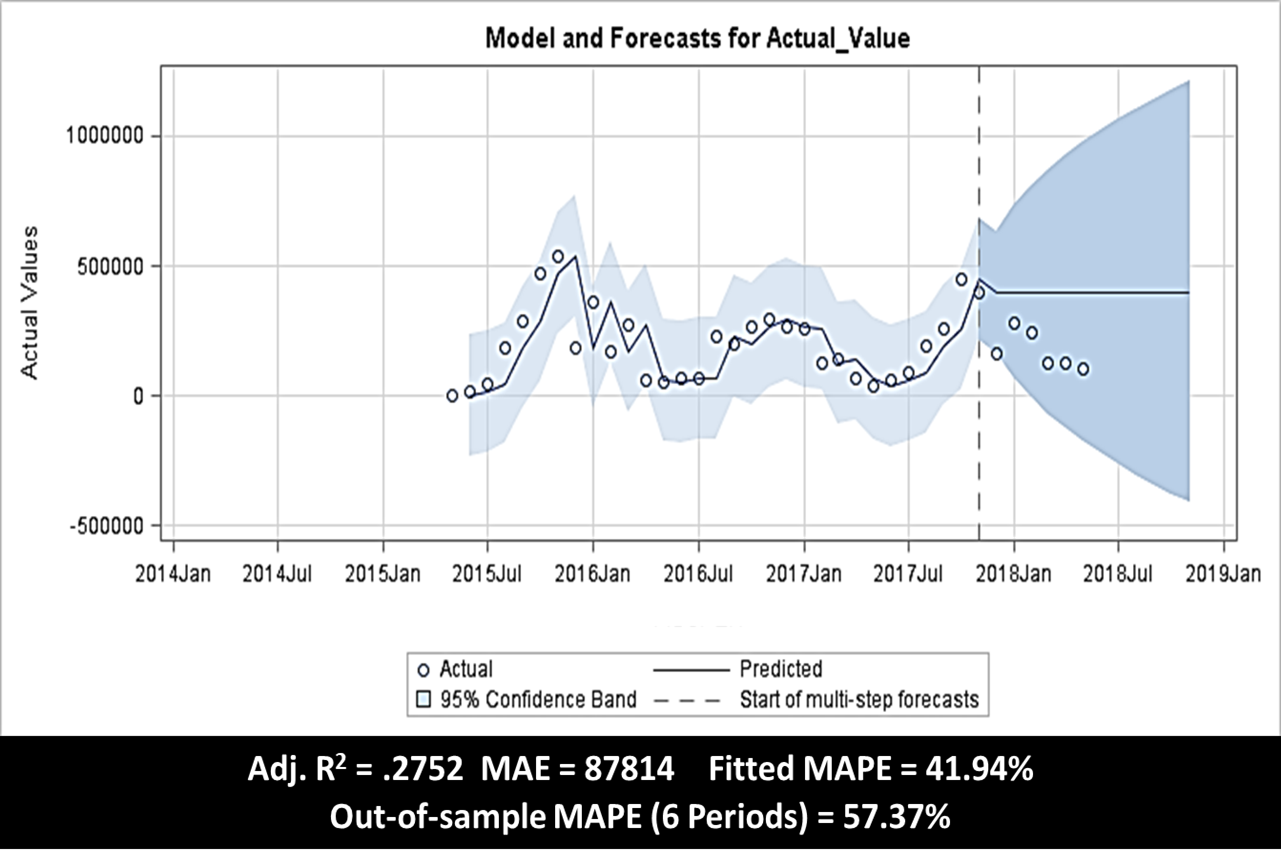
The senior management team at this company didn’t buy into the simple exponential smoothing model’s future forecast based on the historical demand. As a result, a demand analyst built a more advanced seasonal ARIMA(X) model with seasonal differencing, a seasonal auto regressive variable (0,0,0 1,1,0) along with two promotional event variables (intervention variables) to automatically capture the lifts associated with an October and November promotion that was offered in 2015 and 2017. The promotions were not offered in 2016, but are planned to be offered in 2018. So, the demand analyst was able to turn off the promotions for 2016 and turn them on for 2018 by creating two event variables. No manual data cleansing required. See Figure 2.

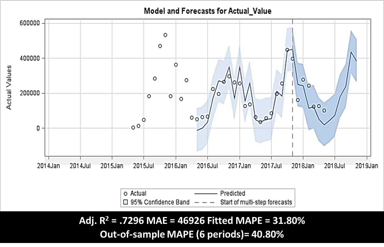
The fitted MAPE using the ARIMAX model was 35.06%, and the out-of-sample MAPE was 40.80%, an improvement over the simple exponential model (ES). The upper/lower future forecast ranges were tighter around the forecast, which could help reduce safety stock.

Also, the MAE (mean absolute error) was significantly improved, as compared to the simple ES model. The MAE was 46.6% lower — decrease from 87814 units to 46926 units. The mean unit reduction from period-to-period could further reduce safety stock.

In Addition, the ARIMA(X) model was able to capture the lifts associated with the October and November promotions, which were 193,821 units and 170,774 units, respectively.  The promotional lifts that were statistically derived by the ARIMA(X) model provided information to Sales/Marketing which lead to the decision to offer those two promotions again in 2018.

Key Learnings

• Forecast accuracy alone is not the only requirement to determine the appropriate method. The future forecast must be salable to senior management.
• Fitted MAPE along with out-of-sample MAPE is a more reliable method to determine the best model versus a fitted MAPE alone.
• Flat-line forecasts with cone shaped upper/lower ranges (95% confidence interval) could have a negative impact on safety stock.
• Only 70%-85% of a product portfolio can be forecasted automatically using an expert system depending on how much causal information is available, as well available demand history.
• Data anomalies along with factors used to influence demand require business acumen along with advanced statistical modeling skills.
  • This requires a demand analytic who has an understanding of sales/marketing programming and strong analytics skills to handle the other 15%-20% of products.

Learn more about large scale automatic statistical forecasting solutions using AI/Machine Learning, and try it out for free.