Mathematical optimization can help business leaders make better decisions in every aspect of their business. After a model has been built, end users are usually interested in doing some sort of scenario analysis to test its robustness and visualizing key performance metrics. SAS has various products that can work with each other to provide a holistic view of the analytical problem. Using SAS Optimization, we can solve myriads of complicated real-world problems, while SAS Visual Analytics allows us to interactively visualize the optimal solution.

In this article, I will provide a demo of a web app that connects SAS Visual Analytics and other SAS® Viya services through REST APIs. The web interface provides an interactive platform to demonstrate small-scale MILP (Mixed Integer Linear Programming) models to non-technical audiences and the ability to perform some scenario analysis by changing certain parameters.The purpose of this demo tool is to enable users with little to no knowledge of SAS programming to invoke the power of SAS Optimization by simply clicking a few buttons.

Since this is a web application project, instead of describing all components of the project I will provide only the sample code of the optimization model, but you may clone my GitHub repository to recreate this project.

High-level Architecture

Server-side library - restaf-server

Everyone with moderate to good front-end coding experience knows the necessity of finding good JavaScript libraries for developing dynamic web applications. The server-side library is restaf-server, which authenticates the connection to a SAS Viya server. It serves up the entry point to the app or the first page and provides the session context to the restaf library.

Front-end library - ReactJS

The restaf library is UI framework agnostic, which means it can be seamlessly integrated into any front-end framework like Angular, React, etc. It provides a user-friendly way to make REST API calls to SAS Viya. A very simple web application showing how to run a small optimization problem and fetch a SAS Visual Analytics report to visualize output using restaf can be found here. In this blog we use the concepts from the simple example to build a much richer application. The UI framework used in this project is ReactJS due to its component-based rendering. ReactJS is easily regarded as the UI framework of choice for most front-end developers and is reportedly being used by all the big companies like Facebook, Uber, Netflix, etc. In fact, it was started by a software engineer at Facebook and has steadily gained popularity. The styling of the web page is done using MaterialUI, which includes styling of the sidebar and the fonts. Some other libraries are also used in this web application, notably, react-bootstrap-table. This library helped me in creating the editable table which ultimately lets the user change input parameters and perform scenario analysis. When you look at the video below, it may seem like a multi-page app. However, it is a misnomer. This app is in fact a single-page app and I am rendering different React components onto the same HTML element. Pretty cool, huh? I am using React Router, another JavaScript library, to enable the routing between the different components.

See below a flowchart of the underlying technologies:

Demo workflow

In this section, I will describe in words the workflow of the Facility Location demo, walk you through each of the interactive components, and demonstrate how the user can do a scenario analysis as well.

But first, check out the video on our YouTube channel for this demo!

Problem Description

Now, let me give you a quick overview of the optimization problem I am trying to demonstrate using the web app. It is a facility location problem for a car manufacturing company. The company has 25 existing facilities, each of which is eligible to produce up to 5 types of cars. The problem is to optimally assign cars to be manufactured at the eligible facilities​. A variable cost is incurred per car manufactured at a facility​, while a fixed cost is a one-time operating cost incurred to keep a facility open or closed​. Each facility can manufacture at most one car. Capacity and demand are also provided in terms of numbers of cars.

Analyze Input Data

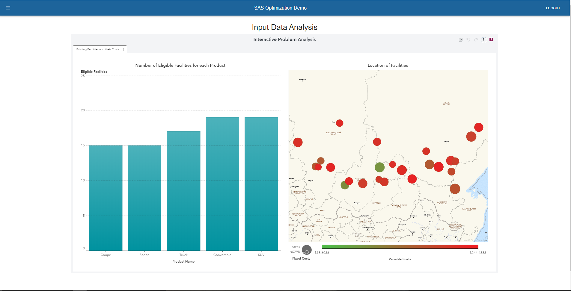
On mounting this component, a SAS Visual Analytics report created by the user on the server to analyze the input data is rendered onto the page. In this report, we can interactively see which facilities are eligible to produce a particular type of car. The bubbles on the map show the different locations of the existing facilities. By clicking on each of the bars, we can filter out the facilities for that type of car. The color of each bubble represents the variable cost for producing a car at that facility and the size of the bubble shows the fixed cost incurred for keeping the facility open. The goal is to select the smallest green bubble for each of the cars.

Input Optimization Parameters

In this component, the user is able to set a few parameters and run the optimization code based on these parameters. They can select the objective function, which can be to minimize fixed costs, variable costs, or total costs​.They may also change the demand for each type of car and/or assign a fixed facility to manufacture it using the editable table. Hitting the 'Optimize' button, a series of promise-based API calls is submitted to the Viya server. First, the updated table from the client-side is passed to the back-end as a JSON object and a table.upload action is used to upload the table to the user's own caslib. Then a string of CASL statements are submitted using the runCASL action, which includes code for the optimization model. Finally, the results are retrieved from the Viya server using REST APIs and the user is redirected to the output report.

Optimization code

The MILP model is coded as a JavaScript string and passed later on into some restAF functions. Anyone with some OPTMODEL experience will easily be able to recognize the syntax in the following code block. It is written as a JavaScript function, which takes the objective type and scenario name as input from the form on the web page. This piece of code, along with a few data pre-processing and post-processing steps, is submitted purely as a string of CASL statements and the 'RunCASL' action is executed using REST APIs.

  function optCode(ObjType, appEnv, scenario) {
  let pgm = `
  set  PRODUCTS;
  set  FACILITIES init {};
  set <str, str> FIXED;
 
  num demand {PRODUCTS};
  num fixed_cost {FACILITIES};
  num close_cost {FACILITIES};
  num x{FACILITIES};
  num y{FACILITIES};
  num var_cost {PRODUCTS, FACILITIES};
  num viable_flg {PRODUCTS, FACILITIES};
  num Obj_Type=${ObjType};
  num capacity {FACILITIES};
  str soln_type init '${scenario}';
 
  read data demandTable into PRODUCTS=[Product_Name] demand;
  read data demandTable  (where = (facility_name ne 'None')) into FIXED=[Product_Name facility_name];
  read data siteTable into FACILITIES=[facility_name] close_cost fixed_cost x y capacity;
  read data costTable into [Product_Name facility_name] var_cost viable_flg;
 
  var Assign {PRODUCTS, FACILITIES} binary;
  var Units {PRODUCTS, FACILITIES} >=0;
  var Close {FACILITIES} binary;
 
  min VarCost
    = sum {i in PRODUCTS, j in FACILITIES} var_cost[i,j]*Units[i,j];
 
  min FixedCost
    = sum {j in FACILITIES} (fixed_cost[j]*(1-Close[j]) + close_cost[j]*Close[j]);
 
  min TotalCost
    = VarCost + FixedCost;
 
  /* Constraints */
 
  /* PRODUCTS demand needs to be satisfied */
  con Demand_Con {i in PRODUCTS}:
    sum {j in FACILITIES} Units[i,j] >= demand[i];
 
  /* each facility have capacity constraints */
  con Capacity_Con2 {j in FACILITIES}:
    sum {i in PRODUCTS} Units[i,j] <= capacity[j]*(1-Close[j]);
 
  /* if operation i assigned to site j, then facility must not be closed at j */
  con If_Used_Then_Not_Closed {j in FACILITIES}:
    sum {i in PRODUCTS} Assign[i,j] = (1-Close[j]);
 
  /*not viable assignemnts*/
  con Viable_Assignemnts {i in PRODUCTS, j in FACILITIES}:
    Assign[i,j] <= viable_flg[i,j];
 
  con Viable_Num_Assignemnts {i in PRODUCTS, j in FACILITIES}:
    Units[i,j] <= capacity[j]*Assign[i,j];
 
  /*Fixing facility - what-if analysis*/
  for{<i,j> in FIXED} fix Units[i,j]=min(demand[i], capacity[j]);
 
  /* solve the MILP */
  if Obj_Type=1 then do;
    solve obj VarCost with milp;
  end;
  else if Obj_Type=2 then do;
    solve obj FixedCost with milp;
  end;
  else if Obj_Type=3 then do;
    solve obj TotalCost with milp;
  end;
 
  /* clean up the solution */
  for {i in PRODUCTS, j in FACILITIES} Assign[i,j] = round(Assign[i,j]);
  for {j in FACILITIES} Close[j] = round(Close[j]);
 
  num siteTotalCost {j in FACILITIES}=
    sum{i in PRODUCTS} var_cost[i,j] * Units[i,j].sol + (fixed_cost[j]*(1-Close[j].sol) + close_cost[j]*Close[j].sol);
 
  num variableCosts{i in PRODUCTS, j in FACILITIES}=
    var_cost[i,j]*Units[i,j].sol;
 
  /* create output */
  create data optimal_cost from
    [product site]={i in PRODUCTS, j in FACILITIES: Assign[i,j] = 1}
    var_cost variableCosts Assign.sol Units.sol;
 
  create data optimal_facilities from
    [site]={j in FACILITIES}
    x y Close.sol siteTotalCost soln_type capacity;
  `;
  return pgm;
}
 
export default optCode;

Analyze Output Report

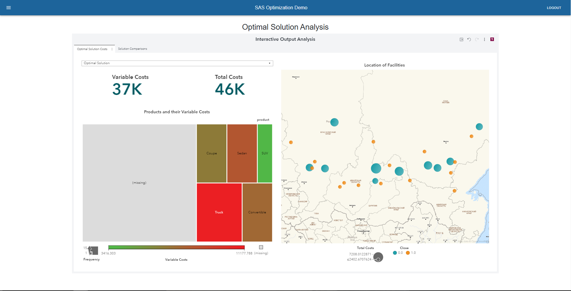
Finally, using React Router I am directly routing the user to the output SAS Visual Analytics report. This report helps visualize the output of the optimization model for each scenario, by showing which facilities to close and which ones to keep open. It also shows the assignment of the products to the facilities, along with the total cost and the variable cost for each scenario. The tree map on the left shows the different products, and the size of each rectangle represents the number of units of each product that is produced. It is connected to the geographic map on the right and enables the user to filter out the facilities for each product. In the next section, I will describe how we can create new scenarios and compare them side by side.

Scenario Analysis

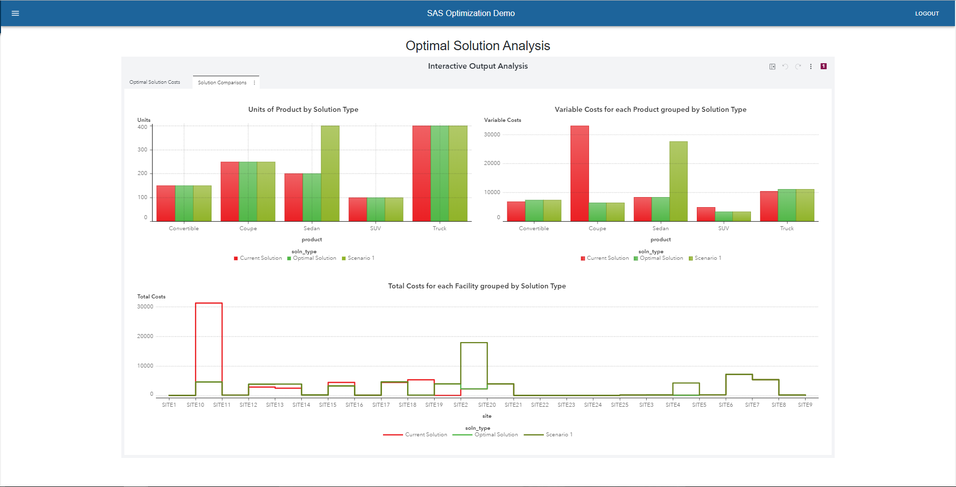
To create a new scenario, the user needs to go back to the 'Input Optimization Parameters' component using the burger menu. A new scenario may be created and the user can either change the number of units required for a product or fix a facility for a product. For the example in the video, I increased the number of units required for Sedan from 200 to 400 and fixed its assignment to Site2. When we analyze the output solutions in the SAS Visual Analytics report, we can see that the total and variable costs for the new scenario increase. The 'Solutions Comparison' tab in the report enables the user to visualize the decisions made by each solution side-by-side. We can see that the variable cost for Sedan has increased due to the increase in number of units. The new solution also requires Site2 to be open, while the optimal solution recommended that it be closed. Similarly, the user can create many more scenarios by giving each scenario a unique name and analyze them in the output report.

What's Next?

Now, that I've shown you how easy it is to combine various SAS products using REST APIs, you can clone my repository and try building one for yourself. The code is sufficiently commented to enable users with some front-end experience to customize it for a different optimization problem. Happy Coding!