Following on from my introductory blog series, Data Science in the Wild, we’re going to start delving into how you can scale up and industrialise your Analytics with SAS Viya. In future blogs we will look at how you can augment your R & Python code to leverage SAS Viya for distributed in-memory analytics. But, before that, we’re going to cover two foundational blog series which introduces core analytics concepts. One on the importance on exploring your data, and another introducing the core concepts of data mining models. Whilst many readers may have a background understanding of analytics already, I feel it is useful to have these primers to make what we discuss open to anyone – and whilst you could just look this information up with your favourite search engine, I personally think it is more helpful to have this all in one place.

It is worth noting that although the examples we use in this series to explore our dataset opt for a (mostly) coding perspective, for everything that we do there is an equivalent way to do it with one of SAS Viya’s unified visual interfaces. For example, in Visual Analytics you can use a correlation plot object, likewise in Model Studio you can use an Explore Data node, etc.

You can find the code for this series here. The SAS code uses ODS to produce an interactive HTHTML output. You can find the source code and HTML output on my GitHub account.

 

 

For completeness this is also presented as a Jupyter notebook visualizing the output. You can export this from the above link and run it directly within your own environment, or simply read through the code. I find this renders better in the JupyterLab interface, but it will work from the standard Jupyter Notebook interface as well. If you want to run the Jupyter notebook, you will need to run the SAS code file first to create the datasets.

 

At the end of this series we’ll also introduce the concept of Visual Exploratory Data Analysis where we’ll reproduce what we’ve already done but from the SAS Visual Analytics interface. In future blogs we’ll have a look at a few different interfaces for SAS Viya using both programmatic and visual capabilities.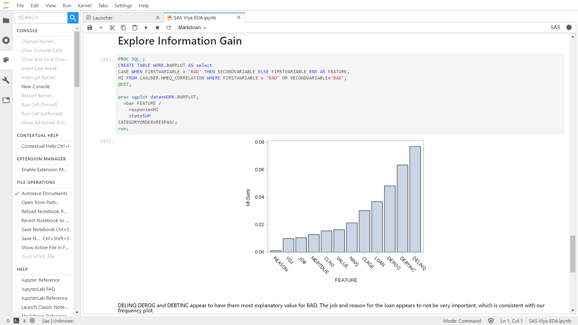

Introduction

Exploratory Data Analysis (EDA) is a really important part of building a robust, reliable, Predictive Model. The proliferation of Machine Learning tools and algorithms has made it very easy to use these techniques without needing to necessarily understand what happens under the hood. Personally, I think this is great, it democratises access to Data Science and enables the Citizen Data Scientist. This allows businesses to upskill existing teams and leverage their own Subject Matter Expertise when working on Data Science initiatives. However, it is important for teams to not rush into building spurious or unreliable models but to instead take the time to really understand their datasets before considering any predictive modelling. As we said in the previous blog series, once you get to know your data well enough, you may not even need a predictive model and the purpose of Data Science is to take an inter-disciplinary approach to understand patterns in your data in order to solve a business problem.

The examples we’ll be showing will be from the HMEQ dataset, a popular open dataset used by data scientists to experiment with Classification modelling techniques.

We won’t be going into how you build a model, however for context if you are new to predictive analytics, a classification model is a model which predicts categorical attributes. In this case the target category is called BAD_CLASS and it is a binary indicator for whether someone has defaulted on their agreed home equity loan amount.

It is important to not only look at the quantitative relationships in the data, but also consider the intuition behind any relationships we find. Below, Table 1 shows a summary of the metadata for the HMEQ dataset. This dataset has been used for Kaggle competitions previously and you can find a nice description of the metadata on the competition page.

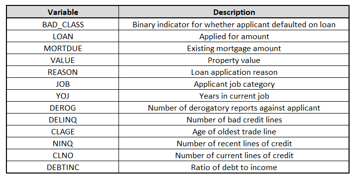
When working with this dataset it important to keep the target class in mind whilst exploring the data. Ask yourself which variables could have an important relationship with whether someone defaults, or is delinquent, on a loan repayment.

For example, before even looking at the dataset it may be reasonable to expect that DEROG and DELINQ have strong relationships with BAD_CLASS as they would appear to be reasonable proxies for credit delinquency. You might also assume that whilst JOB could be a useful indicator, YOJ might not be – as it does not give any indication of overall work experience and might not be a reliable indicator. In a real-life dataset, you might at this point look into gathering any additional fields or datasets which might further augment this. For example, in JOB you might complement it with Years of Experience, Education Level and perhaps derive a ratio of Number of Jobs by Total Experience as an indication of an applicant’s churn rate.

We won’t be going into the details of which models to use, or how to build a model, as we will do this in the next series. Instead we will be looking at our data in order to understand its key drivers and which model inputs might have a strong explanatory relationship with our target BAD_CLASS.

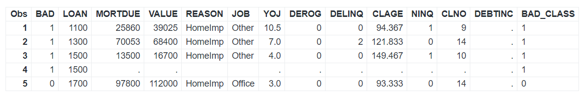
We’ll finish this blog with a snapshot of a few records via PROC PRINT. It is useful to have a quick eyeball of a dataset prior to doing anything else just to ensure that the data look reasonable. Table 2 shows that just looking at the initial snapshot it is clear that there are mostly numeric inputs with varying scales and there are some categorical attributes. The dataset looks reasonably complete but there are clearly cases of missing records which appears to affect rows to a varying degree, we will need to explore the pattern of this missingness as well as assessing the relationships of the inputs against BAD_CLASS.

Please also check out the work of fellow data scientists on model management/skill areas on Data Science Experience hub.