Authors: Steven Harenberg and Amy Becker
The total solar eclipse taking place across a thin band of the United States on April 8, 2024, is going to be a stellar event. In this post, we will help plan a journey to see the total solar eclipse. We will use algorithms available in the NETWORK procedure and action set in SAS Viya to solve various path problems over the United States road network.
A total eclipse is a truly rare and special event, occurring only about once every 18 months somewhere in the world. Each occurrence produces a narrow viewing path, and this year, the path of totality spans a thin band of roughly 110 miles wide, stretching from Mexico to the northeast of the United States and southeast of Canada. The next total solar eclipse that will be seen from the contiguous United States will not be until the year 2044. In short, this is a once-in-a-lifetime event that you do not want to miss!
The closer you are to the center of the path of totality, the more unique and awe-inspiring your experience will be. You will be in the complete shadow of the moon, called the umbra, and witness the cool features that happen only during the total eclipse. Outside of this path of totality, you will see a partial eclipse. It's literally a night and day difference.
Unless you live inside the path of totality, you will have to travel to see the total eclipse. Fortunately, we have the SAS Network Action Set, a powerful tool that can help you plan your journey to view this magnificent event. This Python notebook has all the necessary components for the following examples, making your planning process easier and more efficient.
Data
Several publicly available data sources can help plan for the journey. The key components for this application are the road network and the geometry representing the path of totality. NASA has shapefiles available that provide the geometries for the path of the totality.
For the road network, map data is from Open Street Maps (OSM), that is made available here under the Open Database License (ODbL). The Python package OSMnx (Boeing, G. 2017) is an open source toolkit for conveniently retrieving, converting, and analyzing OSM data as graphs. Check out this Python notebook for more details related to OSM and some other examples.
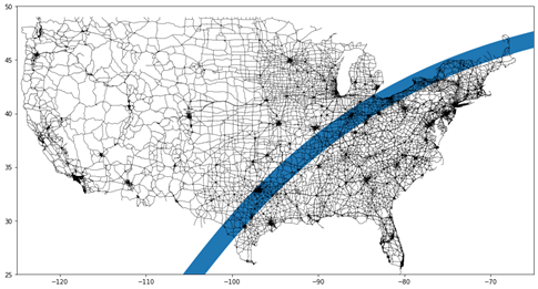
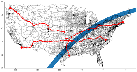
Because we are examining a large-scale routing problem, we do not include residential streets in our road network. We ultimately end up with a network that yields 476,137 nodes and 799,057 links. Each link represents a road, and each node represents an intersection or a dead end. The path of totality and the road network are visualized together in Figure 1.
Finding the shortest path to totality
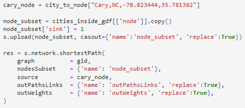
We will start our analysis with possibly the most important question: What is the closest spot from which we can view the total eclipse? To solve this, we start by using the shortestPath action in the network Action Set to compute the shortest paths from SAS headquarters in Cary, North Carolina, to all cities in the path of totality. To do this, we set our source node as Cary, NC, and our sink node as every city that is inside the path of totality (around 2,500 cities). The code for this action call is shown in Figure 2 and available in the Python notebook. Then, from the results in the outWeights table produced by the action, we can find the sink node that has the smallest total travel time.
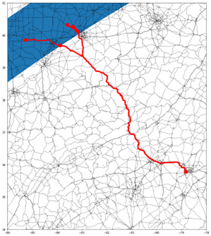
We find that Wilberforce, OH, is the closest such city to Cary, with a total drive time of 7.5 hours. Unsurprisingly, this spot only has a 60-second total eclipse duration because it's the closest point near the edge of totality. This meager duration doesn't cut it for a once-in-a-lifetime event. The NASA eclipse data include geometries for eight duration thresholds from 30 seconds to 240 seconds in 30-second increments. So, we can calculate the shortest path to cities at different duration thresholds to see what other options we have. These routes are summarized in Table 1 and visualized in Figure 3. Excitingly, we discover that with only 30 more minutes of driving, we can end up in a position where we will have a much longer eclipse duration!
| Location | Travel Time (hrs) | Total Eclipse Duration (s) |
| New Lisbon, IN | 8.86 | 240 |
| West Mansfield, OH | 8.05 | 210 |
| Magnetic Springs, OH | 7.85 | 180 |
| Marysville, OH | 7.80 | 150 |
| New California, OH | 7.69 | 120 |
| Dublin, OH | 7.61 | 90 |
| Wilberforce, OH | 7.52 | 60 |
| Cedarville, OH | 7.53 | 30 |
Table 1: Closest point to Cary, NC at different eclipse duration thresholds (summary of the outWeights table produced by the shortestPath action)
Routing for family and friends
Network analytics can also be useful for planning a trip with family and friends. Suppose we want to figure out the best meeting spot for a group of people to gather to watch the total eclipse together. The difficulty is that all these people are spread across the United States. With the shortestPath action, we can specify multiple source and sink nodes to quickly find the shortest paths from each person’s location to all cities in the path of totality. Then, we can aggregate the results to find the best spot based on travel time. One aggregation method that could make sense is to find the sink node that has the smallest maximum travel time for any person to limit the amount of time that any one person must drive.
For example, suppose we need to find a meeting spot for people at the following locations: Cary, NC; Houston, TX; Seattle, WA; San Diego, CA; and Boston, MA. Setting these as source nodes, the outWeights table produced by the shortestPath action gives us travel times for each of these nodes to each city experiencing totality. Aggregating by sink node, we find that Greenwood, AR is the city with the shortest driving time from all starting nodes. The longest any person will have to drive is 29.7 hours from Seattle, and the shortest time any person will have to drive is 7.8 hours from Houston. The set of routes is shown in Figure 4.
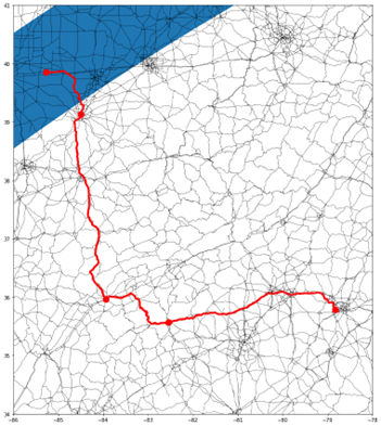
Another useful feature of the shortestPath action is that you can use the sequence parameter to specify a sequence of nodes that must be visited. Suppose we could not convince our friends to drive over 20 hours to the group meeting spot. So instead, we went to New Lisbon, IN, which is the closest location to us at the maximum eclipse duration. We can still make some stops to see friends on the way as we travel to our final destination. Of course, we need a new route to accommodate these extra stops, which we can find by using the shortestPath action with the sequence parameter and specifying the sequence in a table that is given as input to the action. For this example, we will use the following sequence: Cary, NC; Asheville, NC; Knoxville, TN; Cincinnati, OH; New Lisbon, IN. This yields a new path to our destination, that takes 11.05 hours (compared to the 8.86-hour direct path we found previously) but hits the required stops on the way, as shown in Figure 5.
Planning visits to other places by using community detection
Most of the routes we have mapped so far have taken us into the Midwest, as this is the closest point to the total eclipse from Cary, NC. However, we are also interested in seeing other potential routes to places in the path of the eclipse. There are many cities, and it would be overwhelming to consider routes to each one individually. Instead, we can use the community action to partition the set of city nodes into groups of nodes and then consider paths to each of these larger regions.
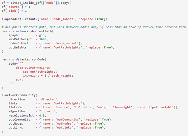
The first step is to run the shortestPath action for all pairs of city nodes that are in totality. The outWeights output table contains travel times between each pair and can be used as input for the community action. We use inverted travel times as edge weights for community detection so that close nodes have a stronger connection than far nodes. The community action will then produce communities where each node in a community is close to the other nodes in that community, effectively giving us regions of cities throughout the band of totality. By tuning the resolution parameter of the community action, we can affect how large or small these regions are depending on the level of granularity we are interested in. The code for these steps is shown in Figure 6.
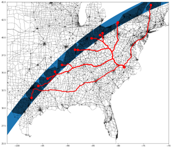
Once we have cities partitioned into communities, we can look at the routes to the node in each community that maximizes the eclipse duration, breaking any ties by using the shortest travel time. Table 2 shows the summary of the routes to each community. We can also use utilities in the GeoPandas package to calculate the convex hull of the nodes in each community and then plot the paths to each representative node of the community, as shown in Figure 7.
| Location | Travel Time (hrs) | Total Eclipse Duration (s) |
| Hewitt, TX | 18.79 | 240 |
| Cumby, TX | 16.60 | 240 |
| Newhope, AR | 15.50 | 240 |
| Springfield, AR | 13.58 | 240 |
| Powhatan, AR | 12.74 | 240 |
| Wayne City, IL | 10.82 | 240 |
| Grayville, IL | 10.40 | 240 |
| New Lisbon, IN | 8.86 | 240 |
| West Mansfield, OH | 8.05 | 210 |
| Caledonia, OH | 8.20 | 210 |
| Erie, PA | 9.45 | 210 |
| McKean, PA | 9.25 | 210 |
| Peru, NY | 12.41 | 210 |
Table 2: Centroid locations of each community ordered by longitude
Conclusion
In this post, we looked at using network analytics in the context of routing problems for the 2024 total solar eclipse. We were able to use publicly available data and open source tools, such as OSMnx and GeoPandas, to build and manipulate road networks that were fed into SAS Network Analytics to perform the main network algorithms. These examples show just a small but extremely powerful set of features that are available in the NETWORK procedure and action set.