When it comes to causal inference, scoring capability is particularly beneficial. It can be used in unique ways that result in an improved decision-making process, such as gaining optimal revenue using the least number of resources. In this post, I will introduce to you a new scoring capability and its use cases with PROC DEEPCAUSAL. I will also show you how it utilizes Deep Neural Networks (DNNs) to perform causal inference as well as policy evaluation and comparison.
The powerful, state-of-the-art and easy-to-use PROC DEEPCAUSAL
Inference is not valid for the estimators when the estimates from machine learning methods are directly plugged into an econometric model. This way creates highly biased estimators, so econometrics methods need to correct for this bias. PROC DEEPCAUSAL does this by implementing the doubly robust estimation method (suggested by Max H. Farrell, Tengyuan Liang, and Sanjog Misra (2021). This method applies DNNs, a powerful machine learning technique, and provides estimates for various causal effect parameters. As well, it performs policy evaluation and policy comparison. DNNs overcome several technical difficulties. These include big data problems, such as high-dimensional covariates; having a mix of discrete or continuous covariates: the unknown nonlinear relationships among the covariates, the outcome, and the treatment assignment. This makes PROC DEEPCAUSAL a very powerful tool for causal inference or analyzing a treatment effect.
PROC DEEPCAUSAL has two main statements for specifying the causal model. First, there is the PSMODEL statement for specifying the propensity score model. Second is the MODEL statement for specifying the outcome model. The propensity score model estimates the treatment by assigning probability conditional on some covariates. The outcome model describes how the outcome depends on the treatment and some covariates. It also consists of two unknown functions, α( ⋅) and β(⋅), that are estimated by a DNN.
If you are wondering what causal inference is, check out this post. It provides preliminary knowledge that makes it easier to understand the concepts explained here.
The new SCORE statement in PROC DEEPCAUSAL
What exactly is scoring? Scoring is the act of producing predictions for a target variable from a predictive model. The benefit of scoring is to avoid the cost of refitting the model when new predictions are needed. Scoring new data to compute predictions for an existing model is a fundamental stage in the analytics life cycle. For example, in industrial process control or monitoring of atmospheric pollutant levels, a sequential data stream is monitored continuously to flag unexpected changes in the normal behavior of the process as soon as possible. Scoring in these situations can be quite useful.
In the context of causal inference, computing predictions for new data or testing the precision of prediction on a test data set are only a part of the advantages of scoring. The scoring capability in causal inference can be useful in many different and important ways that I will be discussing in the next sections.
You can access all the benefits of scoring capability in PROC DEEPCAUSAL by using the recently added SCORE statement.
Let’s look at an example that demonstrates the various advantages of PROC DEEPCAUSAL scoring capability. The causal model in this example is an online music subscription service estimating the effect of targeted customer discounts on the company’s revenue.
The original data set is provided by the Microsoft research project ALICE. For more details, see Example 14.2 in the PROC DEEPCAUSAL documentation. The data are synthetically generated to protect the privacy of the company, but the model variable names and their meanings are preserved. The data have 10,000 observations and include customers’ personal characteristics, such as age and log-income. The data also includes online behavior history, such as previous purchases and previous online times per week. The treatment variable t is the binary variable of whether or not the discount is applied. The output variable is revenue. Table 1 shows the names of the variables that are used in the model, their types, and their definitions.
| Name | Variable Type | Details |
| account_age | covariate | User’s account age |
| age | covariate | User’s age |
| avg_hours | covariate | Average number of hours user was online per week in the past |
| days_visited | covariate | Average number of days user visited website per week in the past |
| friend_count | covariate | Number of friends user connected to in account |
| has_membership | covariate | Whether user has membership |
| is_US | covariate | Whether user accesses website from US |
| songs_purchased | covariate | Average number of songs user purchased per week in the past |
| income | covariate | User’s income |
| t | treatment | Whether a discount is applied |
| revenue | outcome | Number of songs purchased during discount season times price paid |
Table 1: Model Variables
The data are split into three data tables - the training, testing, and “new” data sets. The “new” data observations for the treatment (discount) and the outcome variables (revenue) are set to missing. So, for these customers, you need to figure out the treatment assignment.
The SAS code below demonstrates how to estimate the treatment effect, that is the effect of discount, and saves the estimation details. These details will be used as input for scoring.
* estimate the treatment effect and save the estimation details; proc deepcausal data=mycas.pricing_sample_train; id rowindex; psmodel t = account_age age avg_hours days_visited friends_count has_membership is_US songs_purchased income / dnn=(nodes=(32 32 32 32) train=(optimizer=(miniBatchSize=500 regL1=0.0001 maxEpochs=32000 algorithm=adam) nthreads=20 seed=12345 recordseed=67890)); model revenue = account_age age avg_hours days_visited friends_count has_membership is_US songs_purchased income / dnn=(nodes=(32 32 32 32) train=(optimizer=(miniBatchSize=500 regL1=0.001 maxEpochs=32000 algorithm=adam) nthreads=20 seed=12345 recordseed=67890)); infer out=mycas.oest outdetails=mycas.odetails; score outps=mycas.outpsdata outa=mycas.outadata outb=mycas.outbdata; run; |
The output from this estimation is below.
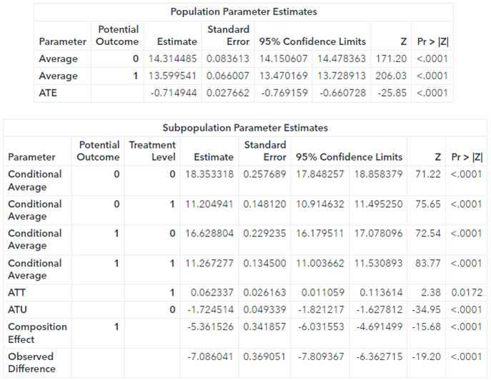
The parameter average potential outcome for an untreated customer is about 14.32, indicating the average effect on the revenue from this customer type. Similarly, the average potential outcome for a treated customer is about 13.6, indicating the average effect on the revenue from this customer type. The parameter ATE (average treatment effect) is usually the main parameter of interest in causal inference. The value of ATE is about -0.72.
This is statistically significant, suggesting that the discount, on average, causes revenue to decrease. However, the estimate for ATT (average treatment effect on the treated) reflects a positive effect of the discount on revenue. The value is small but significant. This could mean that the discount was given to some customers who didn’t care about it. Or the discount wasn’t given to some customers who would have used it. Identifying the characteristics of customers to whom the discount matters helps construct the optimum policy to use the least amount of resources to gain the most profit. The scoring ability can help with this quite efficiently.
Scoring on testing data
Testing the precision of prediction is important. However, in the causal inference context, two other points are also important to consider. The first would be making sure that the observations in the two data sets are coming from the same data generating process (DGP). This would help you understand whether the two policies are the same or not. The second would be to see if there are any outliers in the new data set. You can use the scoring capability of PROC DEEPCAUSAL to handle these three important points. This is how the SAS code might look.
* scoring 1: on testing data: * (1) testing prediction precision (for outcome of regression or treatment of classification); * (2) finding out whether the DGPs are the same (e.g., is there a policy difference?) and the outliers; proc deepcausal data=mycas.pricing_sample_test; id rowindex; infer out=mycas.oest2 outdetails=mycas.odetails2; score inps=mycas.outpsdata ina=mycas.outadata inb=mycas.outbdata; run; |
Note that the MODEL and PSMODEL statements are not included. With the SCORE statement, the model estimation information is already included. So, there is no need to reestimate the model. This saves you a considerable amount of time.
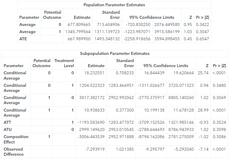
The results are interesting. The estimates for the ATE and many of the other parameters are completely different for the test data set as compared to the training data set. In fact, they are so “off” that it’s hard to make sense out of them. What is going on? There are two explanations for this. Either the two data sets are not generated from the same DGP or there are some outliers. As I mentioned before, this example uses simulated data, eliminating the first possibility. So, there must be some outliers. You can easily identify and eliminate them. Then you can confirm that scoring again produces more similar results to those obtained using the training data set.
Scoring for determining the treatment of new customers
So how would you deal with new customers? How would you determine whether to give them a discount or not given the characteristics that you observe about them?
The third data set contains the information for these new customers. Note that the new observations are missing the outcome and the treatment variable values. Therefore, it is impossible to incorporate the new data into the existing one and reestimate the model. However, we can still use these data to determine who receives the discount and who doesn’t by using the score action of the aStore action set.
One way of approaching this problem is to follow the existing policy we observed in the data set. For this, you can use the analytic store for the propensity score model, outpsdata, that is generated using the OUTPS= option in the SCORE statement during the first call to PROC DEEPCAUSAL. Then calculate the logit of the transformed propensity score and construct a policy based on this propensity score. The SAS code might look like this.
* Scoring 2: Determine the treatment on new customers; * 1) follow the existing policy; proc cas; aStore.score / table="pricing_sample_new_customers" rstore="outpsdata" casout={name="oldway",replace=true} copyvars={"rowindex"}; quit; data oldway; set mycas.oldway; call streaminit(12345); u = rand("uniform"); t_old = (u <= (1/(1+exp(-P_t)))); run; |
However, this approach does not necessarily optimize the revenue from these new customers. The optimum policy, the one that maximizes the revenue, should always lead to a positive treatment effect. In our framework, this translates into treating everyone whose Individual Treatment Effect (ITE) is positive. The function β(x) measures ITE and this function is unknown. Therefore, in practice, an estimate of it is used. This, in effect, translates into a policy giving discounts to those whose predicted beta values are positive. For this, you can use the astore for the information for the beta function estimation, outbdata (similarly generated using the OUTB= option), and create a new policy variable that takes the value of 1 if the predicted revenue for these new customers is positive and the value 0 if it is negative.
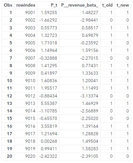
* 2) optimize the policy; proc cas; aStore.score / table="pricing_sample_new_customers" rstore="outbdata" casout={name="newway",replace=true} copyvars={"rowindex"}; quit; data newway; set mycas.newway; t_new = ((P__revenue_beta_) > 0); run; |
The last two columns of Table 2 show the resulting two policies, t_old and t_new, which is also the optimal policy, for the first 20 observations.
The design of this optimal policy runs into the problem of interpretability. The function β(x) is unknown, and a DNN is used to obtain an estimate for it. It’s not known how individual covariates affect the design of the policy. This interpretability issue might be a problem, particularly for policymakers at the government level. In practice, the optimized policy should be as simple as possible and easily explainable. It’s better to use just a small subset of the covariates and easy-to-follow rules. Of course, this raises the question of which subset. Fortunately, the scoring capability of PROC DEEPCAUSAL can help!
Scoring for policy evaluation/comparison/optimization
The optimal policy in application, that is giving discounts to customers for whom _BETA_ is positive, is hard to beat. But at least you can come up with a policy that can come close to the optimal policy and is interpretable. Consider a way of doing personalized discounts based on income. Let’s say you’d like to target customers with the log-income level of at least a threshold level that you pick, say, values starting from 0 to 6.25 by 0.25 increments. Here are the data steps that take care of creating this set of policies.
* scoring 3: policy learning, the evaluation and comparison; * create policies based on income; data mycas.discountPolicy_income; set mycas.odetails; array pi[26] pi0 - pi25; do k = 1 to 26; pi[k] = (income <= 0.25*(k-1)); end; t_opt = (_beta_>0); keep rowindex id t account_age age avg_hours days_visited friends_count has_membership is_US songs_purchased income revenue pi0-pi25 t_opt; run; proc deepcausal data=mycas.discountPolicy_income; id id; infer policy=(t_opt pi0-pi25) policyComparison=(base=(t_opt) compare=(t pi0-pi25)) out=mycas.oest4 outdetails=mycas.odetails4; score inps=mycas.outpsdata ina=mycas.outadata inb=mycas.outbdata; run; |
There are 26 policies, pi0 through pi25. Policies pi0 and pi25 have special meanings. Policy pi0 corresponds to the policy of giving no discount, as no one’s income is less than 0. Policy pi25 corresponds to giving a discount to everyone, as everyone in this data set has income less than 6.25. Now you can run PROC DEEPCAUSAL including this new set of policies in the POLICY= option in the INFER statement. Naturally, comparing this policy with the optimal policy is desired, therefore, t_opt, the optimal policy, is specified in the BASE= suboption of the POLICYCOMPARISON= option. For policy comparison, a negative value for a given policy indicates that it achieves a worse result than the base policy, and a value close to 0 indicates that it is very similar to the base policy. A plot of policy evaluation output is in Figure 1.
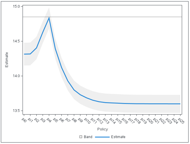
The policy pi4 is almost as good as the optimal policy. Policy pi4 corresponds to threshold 1, that is the policy to provide discounts to customers whose log-income is less than or equal to 1. An important advantage of the policy pi4 is its easy interpretability, unlike the optimal policy.
So, can we do even better? Can we find another set of policies that can outperform pi4 and come even closer to the optimal policy t_opt? This is where the scoring capability comes in handy (again). You can try various sets of policies and compare them with the optimal policy as the base policy by using the POLICYCOMPARISON= option. Thanks to the SCORE statement, each call to PROC DEEPCAUSAL takes only seconds!
Conclusion
Hopefully, you can now see how the scoring capability of PROC DEEPCAUSAL can contribute to making better business decisions. In the causal inference framework, the scoring extends beyond testing prediction. You can also benefit from the scoring capability in many ways that are unique to causal inference. As I demonstrated, you could use it for checking the data accuracy. You can determine if the observations from the two data sets come from the same DGP as well as uncover potential outliers.
I also showed how you can use scoring to determine the treatment on completely new observations. As well, you can also use it for policy evaluation, comparison, and optimization. The latter advantage is particularly important for businesses. They are increasingly interested in understanding the different responses from customers so they can tailor their actions to the customer's needs. Understanding customer characteristics helps businesses to construct policies that use the least number of resources to optimize revenue. The scoring capability in PROC DEEPCAUSAL can most definitely help with that goal.