
In this post, I will introduce the new DEEPCAUSAL procedure in SAS Econometrics for causal inference and policy evaluation. It was introduced in the 2021.1.4 release of SAS Viya 4. First, I review causal modeling and its challenges. Second, I discuss how machine learning techniques embedded in the semiparametric framework can help us to overcome some of these difficulties. Finally, I demonstrate the powerful and easy-to-use PROC DEEPCAUSAL.
Overview of causal inference
Cause-and-effect relationships have been puzzling humans for centuries. Which came first – the chicken or the egg? Whenever you ask why or what-if questions, you are indirectly trying to find answers about cause and effect. The causal inference can help you in your effort. It is the new science of providing the methods and tools for identifying the cause and measuring the effect.
In measuring the causal effect, the randomized experiment is always the gold standard. However, in most cases, the randomized experiment is too expensive or even impossible to conduct. For example, if you would like to know the effect smoking has on developing lung cancer, you can’t randomly assign someone to smoke. If you would like to know how having a college degree affects salary, you can’t randomly send someone to college. In real life, most causal analysis is based on observational data!
Big-data challenge and machine learning tools
Before discussing the challenges of estimating causal effects based on observational data, let’s first focus on the data itself. In the era of big data, it’s not surprising to see tens of or even hundreds of thousands of variables that are used to describe an object of interest (customer, patient, area, store). Some of those variables are often categorical (gender, race), count (number of siblings), or continuous (spending amount on a product last year). In this scenario, two variables are our main interests. They are the outcome variable, denoted as \(\mathit{Y}\), and the treatment variable, denoted as \(\mathit{T}\). For instance, in some personalized pricing cases, \(\mathit{Y}\) could represent demand, and \(\mathit{T}\) could represent whether a discount was offered or not. The causal model is typically researching the relationship between these two variables.
Later in this post, we will discuss the other variables (denoted as \(\mathit{X}\)) which might also be critical in the causal effect estimation. However, how to incorporate those high-dimensional mixed-discrete-and-continuous variables (\(\mathit{X}\)) into the estimation, especially when the relationship between all these variables might be in some unknown nonlinear forms is challenging. The classical linear regressions and the Generalized Linear Models might lead to misspecification. So, we might need some more powerful nonparametric tools. Due to the high dimensionality of the problem, using machine learning or deep learning tools might also be a good idea.
Causation is more than a prediction
Using machine learning and deep learning techniques certainly sounds promising. However, we might not be able to directly apply them in the causal effect estimation. Machine learning is suitable for prediction. Unfortunately, causation is more than a prediction. In the simplest and most common case, the treatment variable is binary. The person is treated or not, and the causal effect is defined as the difference between the potential outcome if the individual were treated,\(\mathit{Y(1)}\), and the potential outcome if the individual were not treated, \(\mathit{Y(0)}\). However, each individual is either treated or not. You can never observe both \(\mathit{Y(1)}\) and \(\mathit{Y(0)}\) for the same individual in the data. This effectively means, \(\mathit{Y(1)} - \mathit{Y(0)} \), the target of your interest, is always missing for all individuals! Hence, we can’t use machine learning tools to directly predict the causal effect.
Instead of estimating the causal effect directly, we can consider breaking the algorithm into three steps. We then use the machine learning tools for the prediction in steps 1 and 2. In step 3, we estimate the average causal effect using results from machine learning steps 1 and 2 as follows:
- We estimate the relationship \(\mathit{f^{(1)}}\)(.) between \(\mathit{X}\) and \(\mathit{Y}\) by using the data of individuals who are treated, \(\mathit{E(Y^{(1)}) = f^{(1)}(X^{(1)})}\), and the relationship \(\mathit{f^{(0)}}\)(.) between \(\mathit{X}\) and \(\mathit{Y}\) by using the data of individuals who are not treated, \(\mathit{E(Y^{(0)}) = f^{(0)}(X^{(0)})}\), where \(\mathit{E}\)(.) is the expectation and \(\mathit{Y^{(T)}}\) and \(\mathit{X^{(T)}}\) denote the data when \(\mathit{T}\) = 0 (untreated) or 1 (treated);
- We predict the \(\mathit{Y}\)(0)s for individuals who are treated by using \(\mathit{f^{(1)}}\)(.) and the \(\mathit{Y}\)(1)s for individuals who are not treated by using \(\mathit{f^{(0)}}\)(.);
- Now, we average the difference between \(\mathit{Y}\)(1)s and \(\mathit{Y}\)(0)s of all individuals and that is the estimated (average) causal effect.
If the data are not observational but comes from random controlled trials, the three-step method above works well. However, when the data are observational, this plug-in method has a good chance to lead to some highly biased estimation results. This is because it does not take care of certain kinds of important variables, known as confounders! The confounders are the variables that have an impact on both the Outcome \(\mathit{Y}\) and Treatment \(\mathit{T}\). Simpson’s Paradox is often used to illustrate the importance of confounders.
For example, in a hospital, 2,050 patients treated for an illness are observed. 550 of them are treated and the rest of the 1,500 are not. 445 patients get cured in the treated group and 1,260 patients get cured in the untreated group. Then, the success rate of the untreated group, 84%, is higher than the success rate of the treated group, 81%. So, this seems that the causal effect is at least nonpositive.
However, when a confounder, the severity of illness (SOI), is considered, an interesting fact is revealed. For patients with higher SOI, the success rate of the treated group is higher than the untreated group. For patients with lower SOI, the success rate of the treated group is also higher than the untreated group! That is, without considering the confounder, we might reach the totally wrong conclusion about the causal effect. The details of the example are shown in Table 1.
| Untreated | Treated | |
| Total | 1260/1500=84% | 445/550=81% |
| Higher SOI | 70/100=70% | 400/500=80% |
| Lower SOI | 1190/1400=85% | 45/50=90% |
Table 1: An example of Simpson’s Paradox
Semiparametric framework comes to the rescue
Now, you know, it’s not easy to estimate the causal effect based on the observational data. This is true even when the machine learning tools can help us to handle the huge number of mixed-discrete-and-continuous variables \(\mathit{X}\), \(\mathit{Y}\) and \(\mathit{T}\), as well as the unknown nonlinear relationships among them. Here, the semiparametric framework comes to the rescue! There are two main steps in the semiparametric framework:
- Nonparametric step: use the machine learning tools (here Deep Neural Networks, DNNs) to estimate the relationship between the treatment variable and the covariates (the so-called propensity score model) and the relationship between the outcome variable and the covariates with the treatment variable (the so-called outcome model).
- Parametric step: for parameters of interest, construct the doubly robust estimator through the influence functions, which takes care of the impact of the confounders.
Among so many machine learning tools, why are DNNs selected? It's because of the DNNs’ convergence rate. One issue that we sometimes experience with machine learning tools in econometrics and other fields is the interpretability of the model. In this particular case, the estimator needs the standard errors to conduct inference. If the machine learning tools can converge to the true unknown functions fast enough in the nonparametric step, the semiparametric framework can provide the valid standard errors of the estimators in the parametric step.
To our knowledge, thanks to the proof in Max H. Farrell, Tengyuan Liang, and Sanjog Misra (2021), DNN is the only machine learning method that can directly fulfill this converge fast requirement. So, by using DNNs in the nonparametric step, we can obtain not only the unbiased estimator but also its standard errors for inference.
The powerful and easy-to-use DEEPCAUSAL procedure
Successfully applying the semiparametric framework including DNN implementation, might not be easy because of the complexity of the estimation. You don’t need to worry, however, because all the technical details are taken care of in the DEEPCAUSAL procedure. For example, the SAS code for estimating the causal effects of interest might look like this:
proc deepcausal data=mycas.mydata; id rowId; psmodel t=x1-x20; model y=x1-x20; infer out=mycas.oest; run; |
In this simple example, no DNN options are needed, because tens of DNN options can take their default values. Of course, if you are an advanced user, you can even specify different DNNs with different training hyperparameters for different models. See the documentation for details.
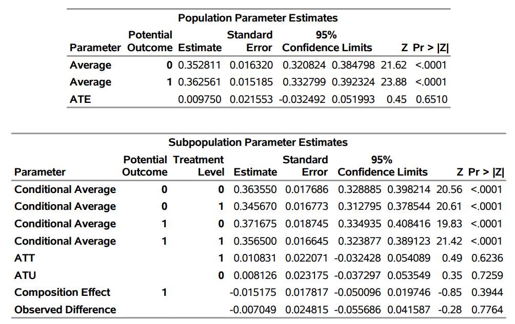
The output of PROC DEEPCAUSAL includes the estimates of parameters of interest for both the full population and the subpopulation. For example, the two most famous and useful parameters of interest are in the output: the average treatment effect (ATE), and the average treatment effect for the treated (ATT). An example of the output from the DEEPCAUSAL procedure is shown in Table 2.
The DEEPCAUSAL procedure and policy evaluation
Besides the parameter estimates, PROC DEEPCAUSAL also supports policy evaluation. which is used to assign the treatment. For example, the policy of sending coupons to customers might be sending them only to customers who spent more than $400 last year. If we know the causal effect on each individual and we can determine the treatment assignment, we have an opportunity to optimize business objectives (maximize revenue, minimize loss, evaluate the impact of a marketing campaign) by setting up the optimal policy.
There are many applications of policy optimization in different fields. Here are just a few: customer targeting, personalized pricing, stratification in clinical trials, learning the click-through rates, and so on. PROC DEEPCAUSAL can evaluate the average effect of a policy or compare the difference between two policies by using the observational data that you have in hand. To do so, you only need to provide the policies in the POLICY= option and the policies to be compared in the POLICYCOMPARISON= option in the INFER statement.
For example, the observational data shows the base policy denoted by t. What if we changed that policy to a new policy denoted by s? Here are two candidates. Policy s1 is to assign treatment to individuals only if their estimated individual treatment effect is positive. The policy s0 is the opposite. It only assigns treatment to individuals whose estimated individual treatment effects are negative. You’d like to evaluate each policy’s average outcome and compare them with the observed treatment t. The SAS code might look like this:
proc deepcausal data=mycas.mydata; id rowId; psmodel t=x1-x20; model y=x1-x20; infer policy=(s1 s0) policyComparison=(base=(t) compare=(s0 s1)) out=mycas.oest; run; |
Table 3 shows the output.
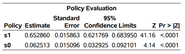
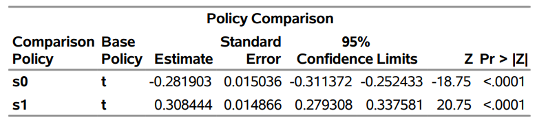
As you can see from the table, different policies have different average outcomes. Policy s1 leads to an average outcome of 0.65 whereas policy s0 leads to an average outcome close to 0. Compared to the observed treatment assignment t, policy s1 has significant positive gains whereas policy s0 has a significant loss. This is an example of where policy matters and why policy optimization is so important.
Other powerful tools for causal inference
Although we covered several topics in this post, there are many more related to causal modeling. The following list mentions a few that might be of interest to you.
- CAUSALGRAPH procedure in SAS/STAT enables you to analyze graphical causal models and to construct sound statistical strategies for causal effect estimation.
- CAUSALMED procedure in SAS/STAT enables you to decompose a (total) causal effect into direct and indirect effects.
- CAUSALTRT procedure in SAS/STAT enables you to perform an estimation of a causal effect.
- MODEL, PANEL, QLIM, and TMODEL procedures in SAS/ETS and the CPANEL and CQLIM procedures in SAS Econometrics support instrumental variables when there are unmeasured confounders.
- PSMATCH procedure in SAS/STAT enables you to perform propensity score analyses and to assess covariate balance.
- VARMAX procedure supports Granger causality tests for time series data.
Causal inference conclusion
Correctly estimating the causal effects is critical for decision-making in our daily lives and business applications, especially in this big data era. In the 2021.1.4 release, SAS provided a new DEEPCAUSAL procedure that takes advantage of both deep learning and econometrics methods and makes your causal inference modeling much easier. We hope you find it useful in your modeling efforts.
LEARN MORE | SAS/STAT LEARN MORE | Deep learning
1 Comment
Pingback: Using PROC DEEPCAUSAL to optimize revenue through policy evaluation - The SAS Data Science Blog