Computer vision is becoming increasingly invaluable in the medical field. It can provide powerful insights into cancer lesion analysis. New computer vision capabilities in SAS Visual Data Mining and Machine Learning (VDMML) can process, analyze and interpret biomedical images to determine biomarkers that can be instrumental in this effort. Likewise, a biomedical image can contain a considerable number of insights into patient health. Consequently, we are continuously seeking new ways to quantify this data and apply it to patient care. In this post, we will be highlighting an important use case from Amsterdam University Medical Center (Amsterdam UMC). We will be applying powerful tools from SAS Visual Data Mining and Machine Learning to assess lesion response to chemotherapy for patients with colorectal liver cancer.
New additions to the BiomedImage action sets
The BiomedImage action sets in SAS Visual Data Mining and Machine Learning provide tools to load, process, and quantify 3D biomedical images. This action set, in combination with others in SAS Visual Data Mining and Machine Learning such as the Image action set, gives you the ability to create powerful end-to-end biomedical image analysis pipelines. New features have recently been added to the BiomedImage action sets to increase efficiency. In particular, a new paradigm has been introduced to the image and BiomedImage action sets to use image-specific parameters. This feature allows you to specify parameters for individual images, rather than using global parameters across all images in the input table. Some examples are image-specific masking and image-specific cropping, which will be discussed in detail later. The addition of these parameters adds another layer of efficiency to image analysis pipelines, as many images can be processed at the same time while utilizing individualized parameters.
Another important addition to the BiomedImage action sets is the ability to calculate the histogram of 3D biomedical images. The histogram of an image represents the frequency distribution of the pixel value data. By using the histogram quantity type in quantifyBioMedImages,you are able to calculate histogram-based metrics that can assist medical professionals with important decisions.
Use case: assessing systemic therapy response with Amsterdam University Medical Center
To demonstrate these new capabilities, consider our customer use case with Amsterdam UMC. In a collaborative effort, SAS and Amsterdam UMC sought to analyze CT scans of patients with colorectal cancer that had spread to the liver. Then we applied these analytics to improve patient treatment. For patients with metastasis spread to the liver, the only way to be cured is surgery to remove the tumors in the liver. This, however, is not always a safe operation to perform. Only about 20% of patients are generally determined to be good candidates for surgery. For the rest of the patients, systemic therapy (including chemotherapy) is first administered to shrink tumors. For these patients, monitoring the effectiveness of these therapies is an important step in determining whether they can then safely undergo a surgical procedure.
Currently, the standard for determining a patient’s response to treatment is to first select two target lesions on the CT scan. Then the changes are measured in the largest diameters of those lesions. Although this criterion is standard practice, this is a very manual process and can be incredibly subjective. The interobserver variability often exceeds 30%. Additionally, by only measuring the 2D diameter of these lesions, a lot of important pixel value information available in these CT scans is being excluded from the analysis.
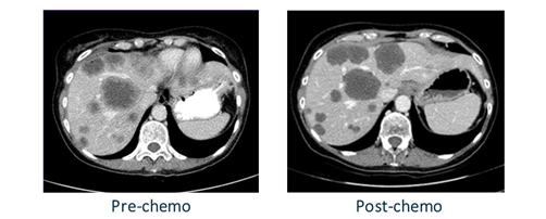
When a patient undergoes chemotherapy, the lesions tend to respond in several different ways that are apparent on CT scans. As seen in figure 1, the lesions tend to shrink, gain more defined borders, and darken in color. Chemotherapy kills the cells of the lesions, causing the regions to become dead scar necrosis. Because of this, these lesion regions tend to be a lot more homogeneous after chemotherapy treatment. This homogeneity is a morphologic response that is correlated with improved patient survival.
In this use case, we seek to capture this important pixel value information and standardize significant biomarkers by using image analysis capabilities in SAS Visual Data Mining and Machine Learning. The data we will be using is from a test set of seven patients that have each undergone one round of chemotherapy. The data contains a 3D CT scan of the patient before and after chemotherapy. As well, we use a corresponding 3D segmentation image that directly labels which pixels within the CT scan are lesions. This segmentation was predicted by a convolutional neural network that had been trained in SAS Viya to identify liver lesions.
Processing the CT scans in SAS Viya
To begin our pipeline, we can first use a new image-specific operation to target regions of the image independently for analysis. Available within the quantifyBioMedImages action, image-specific masking is an invaluable operation for processing biomedical segmentation images. With this operation, you can utilize a region of interest to mask portions of the image that they do not seek to analyze.
# Use image-specific masking to mask the CT scans s.biomedimage.processbiomedimages( images=dict(table="images_with_segmentations"), steps=[ dict( stepparameters=dict( steptype="binary_operation", binaryoperation=dict( binaryoperationtype="mask_specific", image="seg", outputBackground=-1000 ) ) ) ], casout= dict(name="masked_lesions", replace="True") |
Using the Amsterdam UMC data, we can mask regions of the image that are not lesions. This is shown in figure 2.
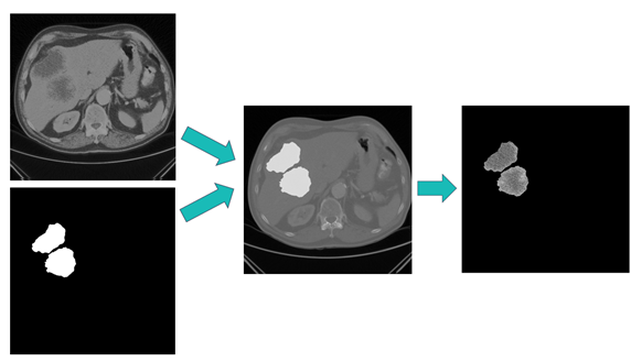
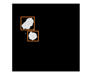
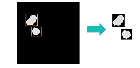
The resulting images contain the original CT scan pixel values in areas of the image that are lesions. All other pixel values are masked to a designated pixel value. Next, each discrete lesion is found within the image by using the boundingBox quantity of quantifyBioMedImages.
# Use quantifyBioMedImages to determine the bounding boxes around lesions in the image s.biomedimage.quantifyBioMedImages( images=dict(table="masked_lesions"), region="component," quantities=[ dict(quantityparameters=dict(quantitytype="boundingbox")), dict(quantityparameters=dict(quantitytype="minimum")), dict(quantityparameters=dict(quantitytype="maximum")), dict(quantityparameters=dict(quantitytype="content", useSpacing=True)) ], inputbackground=-1000, labelParameters=dict(labelType="basic", connectivity="vertex"), casout=dict(name="lesion_bounding_boxes", replace="True") ) |
Note that by setting the region parameter to the value “component”, this action will quantify each connected component separately within the images. The components are quantified based on several different metrics. The boundingbox quantity is specified to determine the location and size of the bounding box for each individual component. This is demonstrated in figure 3.
After we determine the bounding box information for each of the individual lesions, we can then utilize this information to crop the lesions into individual images.
# Crop each lesion region by using the bounding box information s.biomedimage.processbiomedimages( images=dict(table="masked_with_bounding_boxes"), steps=[ dict( stepparameters=dict( steptype="crop", cropparameters=dict(croptype="specific") ) ) ], casout=dict(name="cropped_lesions", replace="True") ) |
This image-specific cropping operation, demonstrated in figure 4, can be accomplished in the processBioMedImages action.
As this new operation avoids the need to use different global cropping parameters for each action call, this introduces a massive performance improvement into the processing pipeline.
Computing histogram-based IBSI metrics
Now that our images are cropped to individual lesions, we can now compute biomarkers for these lesions to track their response to therapy. Accordingly, the Image Biomarker Standardization Initiative (IBSI) provides some standard histogram-based metrics that we can use to assess these pixel value changes. The addition of histogram calculation in quantifyBioMedImages is integral to calculating these metrics.
# Define the histogram parameters number_of_bins = 32 histogram_min = -100 histogram_max = 400 # Calculate the histogram of each lesion region s.biomedimage.quantifybiomedimages( images=dict(table="cropped_lesions"), quantities=[dict( quantityparameters=dict( quantitytype="histogram", bins=number_of_bins, min=histogram_min, max=histogram_max ) ), ], casout=dict(name="lesion_histogram", replace="True") ) |
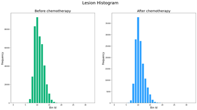
As shown in this code snippet, you can specify the histogram quantity type in quantifyBioMedImages to calculate the histogram for each of the lesion regions. In figure 5, we can observe some of the differences between the lesion histogram before and after chemotherapy. For example, the histogram of the lesion after it has undergone chemotherapy has a steeper peak and less spread than the pre-chemo histogram. This post-chemo histogram has also shifted left, indicating that the pixel values are darker after undergoing therapy.
Now that the histogram is computed for each lesion within the test set, we can calculate the IBSI metrics for these histograms. This can be done in several ways. But in this instance, we use computedvars to define programs to calculate each of the metrics by using the output histogram table columns. The view action is then called to execute these programs. Table 1 displays the histogram metrics that were computed for the same lesion that was used in the histogram visualization.
| Mean | Kurtosis | Variance | Uniformity | Skewness | Standard Deviation | |
| Lesion before chemotherapy | 10.780624 | -0.001799 | 3.403466 | 0.157620 | 5.531227 | 1.844848 |
| Lesion after chemotherapy | 10.724724 | 0.720284 | 3.326845 | 0.171053 | 6.785664 | 1.823964 |
Here, we can see a few different indicators on how this lesion is responding to treatment. In general, these metrics indicate that the lesion is getting darker and the pixel values are becoming more homogeneous. Consider the kurtosis metric, which measures the peakedness of a distribution. A negative kurtosis indicates that the distribution is very spread. A positive kurtosis indicates that the pixel values are converging and becoming more similar. As the kurtosis of this lesion’s histogram changes from negative to positive after chemotherapy, we can determine that the lesion is responding to the therapy. Now, let us look at all the lesions within a patient’s CT scan and calculate the metrics for these regions as a whole. In figure 6, the mean of the lesion regions for each patient is plotted before and after chemotherapy.
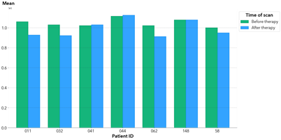
Interpreting these results, we can see the mean tends to drop after the patient undergoes chemotherapy. This is expected, as pixels of the lesion region often darken after chemotherapy. This might indicate that the patients, in general, are responding to the therapy. By deriving these metrics automatically, medical professionals have more data points without having the laborious task of manipulating the images individually. These insights provide patients with more personalized care and well-informed decisions about their treatment.
Conclusion
Computer vision is increasingly gaining traction in the medical field. It will continue to advance patient care and medical outcomes in the years ahead. The information available within biomedical images is immense. If utilized it can provide a deeper insight into personalized care for patients. With continuous improvements in SAS Viya, we are consistently gaining new abilities to process and analyze patient images for a better future. These powerful tools can assist with important decisions in the clinic. They can even help determine whether a patient can receive life-saving surgery.
Learn more | Medical Image Analysis in SAS Viya Learn more | Automatic Spinal Cord Segmentation