Note from Udo Sglavo: The 2021 Nobel Prize for Economics was awarded to David Card, Joshua Angrist, and Guido Imbens. In this post, I discuss their achievements with Xilong Chen, Senior Manager of Econometric Modeling at SAS. Following cutting-edge research and embedding it into our software to benefit our users is always at the top of our priorities list. I am excited to discuss with Xilong how the Nobel Prize winner’s research is reflected in our causal econometrics and statistical modeling software.

Udo: I heard that this year’s Nobel Prize for Economics is related to causal econometrics. Could you tell me more?

Xilong: This year’s Nobel Prize for Economics was awarded to David Card “for his empirical contributions to labor economics”, and to Joshua Angrist and Guido Imbens “for their methodological contributions to the analysis of causal relationships.” They are all related to answering causal questions using observational data.

Udo: How are Card’s contributions related to causal econometrics?

Xilong: Card used natural experiments to study labor economics problems in the 1990s. For example, Card and Krueger (1994) answered the question of what the effect is of increasing the minimum wage on the employment rate using causal econometrics approaches.

Udo: Can you tell us more about Card’s methodology?

Xilong: Studying cause-effect problems is not necessarily easy because you can’t freely conduct random experiments. For example, if you could randomly increase some areas’ minimum wages and keep other areas’ minimum wages unchanged across the whole country, it would be easy to find the causal effect. It would just be a difference between the average employment of the areas where the minimum wage is increased (the treated group) and that of the areas where the minimum wage is unchanged (the control group). Random experiments would be ideal for causal effect estimation. However, these kinds of random experiments, especially in social studies, cannot be executed because they are too expensive, unethical, or simply impossible to set up.

Udo: I understand that obtaining data from random experiments would be difficult. Can you tell us how Card did it?

Xilong: He relied on observational data (from what he called natural experiments) to estimate the causal effect. Natural experiments set up the environment just like random experiments. However, the experiment is not specifically designed to research a particular topic. It just happens as a coproduct of another action. Just like in random experiments, the treatment group and control group match each other in all other factors or variables except the treatment and the outcome.

These “experiments” often happen due to policy changes, natural or institutional events. Card exploited the data from the fast-food restaurants near the border between New Jersey and Pennsylvania. It happened when New Jersey increased the minimum wage, but Pennsylvania didn’t. Then, the comparison of employment change between the restaurants in two states answered the causal question of whether the minimum wage increase decreased employment. This approach was a truly unique challenging standard textbook model at the time.

Udo: Are the methodological contributions to the analysis of causal relationships by Angrist and Imbens also based on the observational data?

Xilong: Yes, they are. In one of my previous blog posts, I mentioned that it’s difficult to estimate the causal effect based on observational data. One main obstacle is how to consider the confounders, which are the variables having an effect on both the treatment assignment and the outcome. In the blog post mentioned, I talked about observable confounders. However, Angrist and Imbens’ main contributions are about the unobservable confounders. If unobservable confounders exist, the instrumental variable approaches should be used. They successfully integrated the instrumental-variable approach and the potential-outcome framework into a new framework, defined assumptions, and pointed out how to estimate and interpret the estimated causal effect.

Udo:  Could you use an example to explain Angrist and Imbens’ main work?

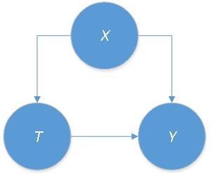
Xilong: A classic example concerns estimating the causal effect of how graduating high school affects wages. In this example, the treatment variable, denoted by T, is whether the individual completes high school or not. The outcome variable, denoted by Y, is the individual’s earnings. If we could run a random experiment, randomly assigning some individuals to a treatment group in which all individuals finish high school, and others to a control group in which all individuals do not finish high school,  we could focus on the treatment and outcome variables. We could also ignore all other variables or factors that describe different individuals or contexts. Then the difference between the two groups’ average outcomes would be the causal effect we are seeking. The causal relationship can be expressed in Figure 1.

Udo: This seems simple and effective, but you mentioned earlier that this approach is not going to work in most situations because we can’t set up a random experiment. Correct?

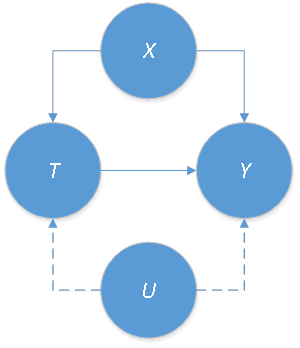
Xilong: Yes, that is correct. We know random experiments can’t be performed in the real world in most cases; we can only use observational data. Then, there might exist some observable confounders, denoted by X; for example, parents’ education level. See the causal graph in Figure 2.

Introducing unobservable confounders

There are several ways to correct the bias introduced by observable confounders X, like the influence functions, regression adjustment, and so on. However, also there often exist confounders that can’t be observed or measured. Examples would be an individual’s “ability”, “motivation”, and/or “willingness to work hard.” Let’s denote the unobservable confounders as U. The new causal graph showing observed and unobserved cofounders is depicted in Figure 3.

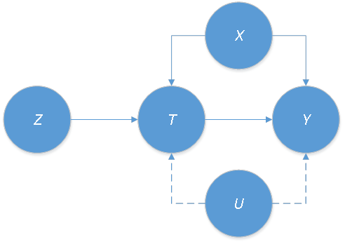
Angrist and Imbens worked on how to correct the bias introduced by the unobserved confounders U. Econometricians often use the instrumental variables, denoted by Z, to solve this problem as depicted in Figure 4.

Combining instrumental-variable framework in econometrics and the potential-outcome framework in statistics

In this cause-and-effect context, the difficult question is what kind of variables can be used as an instrumental variable? Then after using instrumental variables and obtaining the estimation, how to interpret the result? Those problems are answered in Angrist and Imbens (1994). They combined the instrumental-variable framework in econometrics and the potential-outcome framework in statistics (proposed by Neyman in 1923 and extended and refined by Rubin in 1974) into a new framework. They gave some clear and simple assumptions. So researchers can apply this new framework to check the instrumental variables. As well as being able to estimate the causal effect even when some confounders are unobservable.

In this specific example, the instrumental variable they used is the quarter in which an individual is born. This is a very surprising variable, right? However, this surprising variable meets the assumptions. For example, it has a direct effect on the decision of completing high school (the assignment of treatment), but it doesn’t directly affect the earnings (the outcome).

Udo: Do we have products to support Card’s, and Angrist, and Imbens’ methods?

Xilong: Yes, by now their methods are well developed and implemented in SAS. We have several procedures in SAS Econometrics to support the instrumental variables when there are unobserved confounders. For example, the well-known method Two-Stage Least Squares (2SLS; see Angrist and Imbens, 1995) is supported in PROC MODEL and PROC TMODEL. For the panel data (or cross-sectional time series data), you can use PROC PANEL and PROC CPANEL. When the range of possible values of an outcome variable is restricted or it is observed in discrete values, you can use PROC QLIM and PROC CQLIM.

Recently, PROC DEEPCAUSAL was made available in the 2021.1.4 release of SAS Viya 4. It introduces the deep learning methods for causal inference and policy evaluation. It is suitable to address the high-dimensional mixed-continuous-and-discrete variables with unknown nonlinear relationships in the big-data world.

At the same time, SAS/STAT also provides lots of procedures, such as PROC CAUSALTRT, PROC CAUSALMED, PROC PSMATCH, and so on, to address different kinds of causal inference problems. In the previous example of the effect of completing high school on earnings, I use the causal graph to show the relationships between variables. PROC CAUSALGRAPH in SAS/STAT enables you to analyze graphical causal models and to construct sound statistical strategies for causal effect estimation.

Udo: What are the plans for future development in the area of causal analyses?

Xilong: We have been working on several new products for causal inference. For example, we’d like to introduce new machine learning tools (besides deep learning methods) into causal inference. Compared to deep learning methods, some other machine learning tools might be faster, less complex with a smaller memory footprint, and even guarantee some asymptotic properties (see Athey and Wager, 2021, for an example).

We are also considering methodologies to address dynamic treatment effects when the interest is on the effect of a sequence of treatments, instead of the static one-time treatment. As mentioned before, PROC CAUSALGRAPH can help you in causal modeling; however, the causal graph must be available before using PROC CAUSALGRAPH. Currently, the causal graph must be provided by some domain expert. In the future, we would like to learn causal relationships (graph) directly from the data. This is called the causal graph discovery.

Udo: How do you envision the future of causal inference?

Xilong: Causal inference is a huge topic. It has been applied not only in econometrics or statistics, but also in AI, machine learning, medicine, social science, and many other fields. There are lots of unsolved problems in causal inference. Every day, there are new methods and algorithms being developed. I  am excited to be part of it. I  truly believe that SAS products play a critical role in helping people answer their causal questions of interest. And solve their business problems!